---
title: "Jansen-Rit Peak Frequency Optimization"
subtitle: "Reproducing MEG Resting-State Frequency Gradients with Network Dynamics"
format:
html:
code-fold: false
toc: true
echo: false
embed-resources: true
fig-width: 8
out-width: "100%"
jupyter: python3
execute:
cache: true
---
Try this notebook interactively:
[Download .ipynb](https://github.com/virtual-twin/tvboptim/blob/main/docs/workflows/JR.ipynb){.btn .btn-primary download="JR.ipynb"}
[Download .qmd](JR.qmd){.btn .btn-secondary download="JR.qmd"}
[Open in Colab](https://colab.research.google.com/github/virtual-twin/tvboptim/blob/main/docs/workflows/JR.ipynb){.btn .btn-warning target="_blank"}
## Introduction
This tutorial demonstrates how to use TVB-Optim's Network Dynamics framework to model and optimize brain network dynamics. We aim to reproduce the frequency gradient observed in resting-state MEG data, where different brain regions exhibit characteristic peak frequencies that vary with their distance from visual cortex.
```{python}
#| output: false
#| echo: false
# Install dependencies if running in Google Colab
try:
import google.colab
print("Running in Google Colab - installing dependencies...")
!pip install -q tvboptim nibabel nilearn
print("✓ Dependencies installed!")
except ImportError:
pass # Not in Colab, assume dependencies are available
```
```{python}
#| output: false
#| echo: true
#| code-fold: true
#| code-summary: "Environment Setup and Imports"
# Set up environment
import os
import time
cpu = True
if cpu:
N = 8
os.environ['XLA_FLAGS'] = f'--xla_force_host_platform_device_count={N}'
# Import all required libraries
import numpy as np
import matplotlib.pyplot as plt
import matplotlib.patheffects as path_effects
import jax
import jax.numpy as jnp
import copy
import equinox as eqx
import optax
from IPython.display import Markdown, display
import pandas as pd
import nibabel as nib
from nilearn import plotting
# Import from tvboptim
from tvboptim import prepare
from tvboptim.types import Parameter, Space, GridAxis
from tvboptim.types.stateutils import show_parameters
from tvboptim.utils import set_cache_path, cache
from tvboptim.execution import ParallelExecution, SequentialExecution
from tvboptim.optim.optax import OptaxOptimizer
from tvboptim.optim.callbacks import MultiCallback, DefaultPrintCallback, SavingCallback, AbstractCallback
# network_dynamics imports
from tvboptim.experimental.network_dynamics import Network, solve, prepare
from tvboptim.experimental.network_dynamics.dynamics.tvb import JansenRit
from tvboptim.experimental.network_dynamics.coupling import LinearCoupling, SigmoidalJansenRit, DelayedSigmoidalJansenRit, AbstractCoupling
from tvboptim.experimental.network_dynamics.graph import DenseGraph, DenseDelayGraph
from tvboptim.experimental.network_dynamics.solvers import Euler, Heun
from tvboptim.experimental.network_dynamics.noise import AdditiveNoise
from tvboptim.data import load_structural_connectivity
from tvboptim.experimental.network_dynamics.utils import print_network
# Set cache path for tvboptim
set_cache_path("./jr")
```
## Loading Structural Data
We load the Desikan-Killiany parcellation atlas and structural connectivity data.
```{python}
#| output: false
#| echo: true
#| code-fold: true
#| code-summary: "Load structural connectivity data"
# Load volume data for visualization
# Try local path first, fall back to GitHub download for Colab
try:
dk_info = pd.read_csv("../data/dk_average/fs_default_freesurfer_idx.csv")
dk = nib.load("../data/dk_average/aparc+aseg-mni_09c.nii.gz")
except FileNotFoundError:
import urllib.request
from pathlib import Path
# Download from GitHub to local cache
cache_dir = Path.home() / ".cache" / "tvboptim" / "dk_average"
cache_dir.mkdir(parents=True, exist_ok=True)
base_url = "https://raw.githubusercontent.com/virtual-twin/tvboptim/main/docs/data/dk_average"
for filename in ["fs_default_freesurfer_idx.csv", "aparc+aseg-mni_09c.nii.gz"]:
local_file = cache_dir / filename
if not local_file.exists():
print(f"Downloading {filename}...")
urllib.request.urlretrieve(f"{base_url}/{filename}", local_file)
dk_info = pd.read_csv(cache_dir / "fs_default_freesurfer_idx.csv")
dk = nib.load(cache_dir / "aparc+aseg-mni_09c.nii.gz")
dk_info.drop_duplicates(subset="freesurfer_idx", inplace=True)
# Load structural connectivity with region labels
weights, lengths, region_labels = load_structural_connectivity(name="dk_average")
```
## Background: Resting State MEG
Experimental studies of resting-state brain activity using MEG have revealed a systematic gradient in oscillatory peak frequencies across cortical regions. Lower-frequency alpha oscillations (~7-8 Hz) dominate in higher-order association areas, while higher frequencies (~10-11 Hz) are observed in sensory cortices. This gradient follows the cortical hierarchy from sensory to association areas.
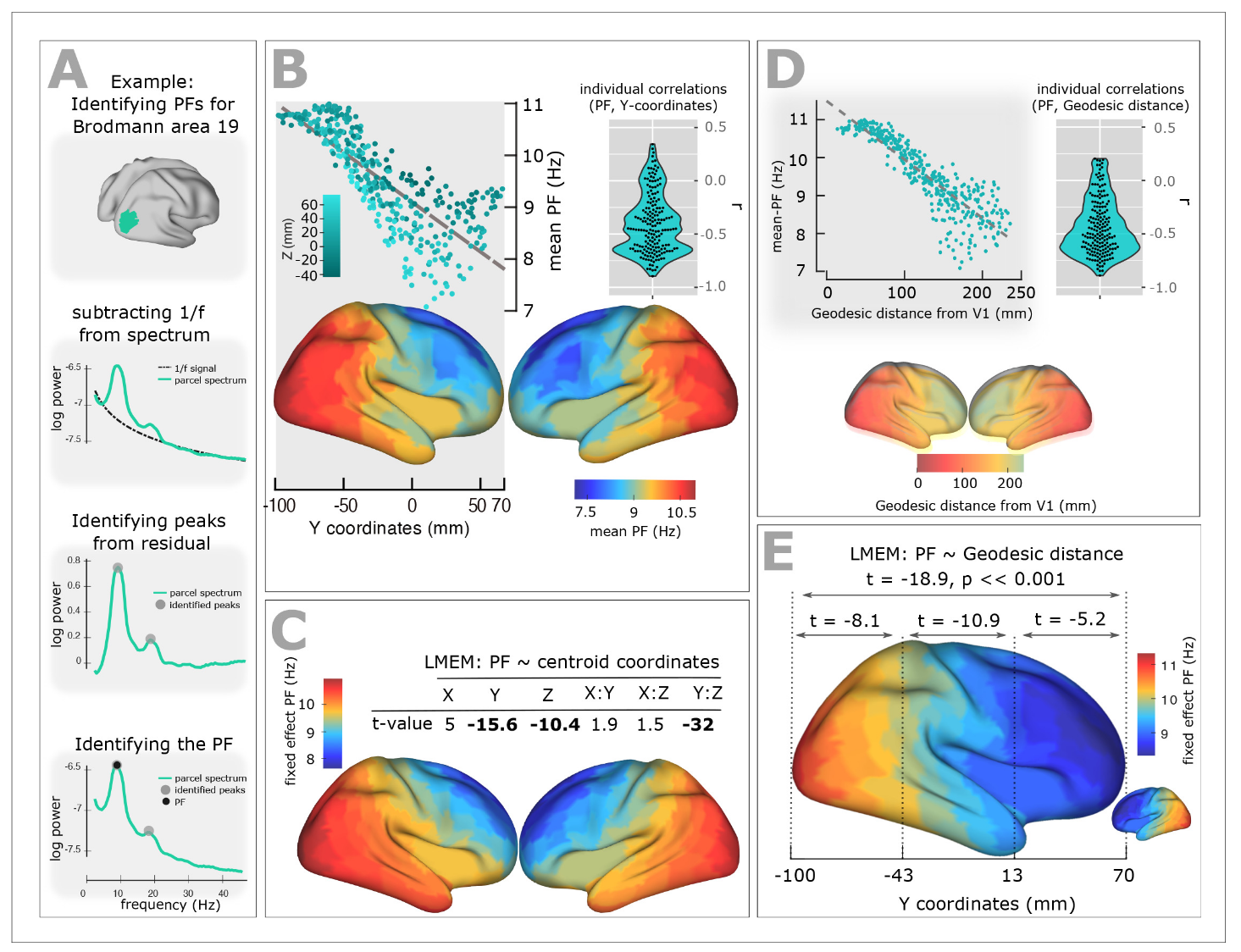{#fig-meg-gradient}
## Defining Target Frequencies
We approximate this gradient by mapping peak frequencies based on the distance from visual cortex (lateral occipital gyrus), ranging from 11 Hz at visual cortex to 7 Hz at the most distant regions.
```{python}
#| output: false
#| echo: true
#| code-fold: true
#| code-summary: "Compute distance-based frequency targets"
ab_map = np.zeros(dk.shape)
# freesurfer index where acronym == name in df dk_info
# Lateral Occipital Gyrus
idx = dk_info[dk_info.acronym == "L.LOG"].freesurfer_idx.values[0]
ab_map = np.where(dk.get_fdata() == idx, 1, ab_map)
idx = dk_info[dk_info.acronym == "R.LOG"].freesurfer_idx.values[0]
ab_map = np.where(dk.get_fdata() == idx, 1, ab_map)
region_labels = np.array(region_labels)
idx_l = np.where(region_labels == "L.LOG")[0]
idx_r = np.where(region_labels == "R.LOG")[0]
dist_from_vc = np.array(np.squeeze(0.5 * (lengths[idx_l, :] + lengths[idx_r, :])))
dist_map = np.zeros(dk.shape)
for name, dist in zip(region_labels, dist_from_vc):
idx = dk_info[dk_info.acronym == name].freesurfer_idx.values[0]
dist_map = np.where(dk.get_fdata() == idx, dist, dist_map)
n_nodes = 84
f_min = 7 # at max distance
f_max = 11 # at VC
min_dist = dist_from_vc.min()
max_dist = dist_from_vc.max()
delta_f = (f_max - f_min) / (max_dist - min_dist)
peak_freqs = f_max - delta_f * (dist_from_vc - min_dist)
f_map_target = np.zeros_like(dk.get_fdata())
for name, fp in zip(region_labels, peak_freqs):
idx = dk_info[dk_info.acronym == name].freesurfer_idx.values[0]
f_map_target = np.where(dk.get_fdata() == idx, fp, f_map_target)
```
```{python}
#| label: fig-distance-visual-cortex
#| warning: false
#| fig-cap: "**Target frequency gradient based on anatomical distance.** Left: White matter fiber tract lengths (mm) from each region to the lateral occipital gyrus (black outline), which approximates visual cortex in the Desikan-Killiany parcellation. Right: Target peak frequencies mapped from distance, with 7 Hz for the most distant regions and 11 Hz for visual cortex."
#| code-fold: true
#| code-summary: "Show plotting code"
# Create figure with two equal-sized subplots
from mpl_toolkits.axes_grid1 import make_axes_locatable
fig, (ax_gb, ax_freq) = plt.subplots(1, 2, figsize=(8.1, 4.05))
# Plot glass brain with distance map
plotting.plot_glass_brain(
nib.Nifti1Image(dist_map, dk.affine),
cmap="cividis",
threshold=0,
title=None,
black_bg=False,
vmin=dist_from_vc.min(), vmax=dist_from_vc.max(),
colorbar=False,
display_mode="z",
axes=ax_gb
)
# Overlay glass brain with anatomical map
plotting.plot_glass_brain(
nib.Nifti1Image(ab_map, dk.affine),
cmap="Greys",
colorbar=False,
threshold=0,
display_mode="z",
axes=ax_gb
)
# Add colorbar for distance map
norm_dist = plt.Normalize(vmin=dist_from_vc.min(), vmax=dist_from_vc.max())
sm_dist = plt.cm.ScalarMappable(cmap="cividis", norm=norm_dist)
sm_dist.set_array([])
# Create colorbar for distance map
divider_gb = make_axes_locatable(ax_gb)
cax_gb = divider_gb.append_axes("left", size="5%", pad=0.5)
cbar_gb = plt.colorbar(sm_dist, cax=cax_gb, orientation="vertical")
cbar_gb.set_label('Distance from visual cortex [mm]')
# Plot frequency map with fixed colorbar range
plotting.plot_glass_brain(
nib.Nifti1Image(f_map_target, dk.affine),
cmap="cividis_r",
threshold=0,
title=None,
black_bg=False,
display_mode="z",
vmin = 6.5,
vmax = 11.5,
axes=ax_freq,
colorbar=False
)
# Add colorbar for frequency map with fixed range from 7 to 11 Hz
norm_freq = plt.Normalize(vmin=6.5, vmax=11.5) # Fixed range from 7-11 Hz
sm_freq = plt.cm.ScalarMappable(cmap="cividis_r", norm=norm_freq)
sm_freq.set_array([])
# Create colorbar for frequency map
divider_freq = make_axes_locatable(ax_freq)
cax_freq = divider_freq.append_axes("right", size="5%", pad=0.5)
cbar_freq = plt.colorbar(sm_freq, cax=cax_freq, orientation="vertical")
cbar_freq.set_label('Target Frequency [Hz]')
# Add panel numbers
# for i, ax in enumerate([cax_gb, ax_freq], start=1):
# panels.add_panel_number(ax, i, text_kwargs={'fontsize': 16, 'fontweight': 'bold', "zorder": -1})
# Finalize figure
fig.tight_layout();
```
## The Jansen-Rit Model
The Jansen-Rit model is a neural mass model that describes the mean activity of interconnected populations of excitatory and inhibitory neurons in a cortical column. It produces realistic alpha-band oscillations and is widely used in whole-brain modeling.
The model has three key rate parameters: `a` and `b` control the time constants of excitatory and inhibitory populations respectively, while `mu` sets the baseline input. These parameters determine the oscillation frequency and amplitude.
```{python}
#| echo: true
#| label: fig-jr-single
#| fig-cap: "**Single Jansen-Rit oscillator dynamics.** Time series showing characteristic alpha-band oscillations with parameters a=0.075 ms⁻¹, b=0.075 ms⁻¹, and μ=0.15."
dynamics = JansenRit(a = 0.075, b = 0.075, mu = 0.15)
dynamics.plot(t1=1000, dt = 1)
```
## Code for the Jansen-Rit Model and Sigmoidal Coupling
```{python}
#| output: false
#| echo: true
#| eval: false
#| code-fold: true
#| code-summary: "View source code for JansenRit and DelayedSigmoidalJansenRit"
class JansenRit(AbstractDynamics):
"""Jansen-Rit model with multi-coupling support."""
STATE_NAMES = ("y0", "y1", "y2", "y3", "y4", "y5")
INITIAL_STATE = (0.0, 5.0, 5.0, 0.0, 0.0, 0.0)
AUXILIARY_NAMES = ("sigm_y1_y2", "sigm_y0_1", "sigm_y0_3")
DEFAULT_PARAMS = Bunch(
A=3.25, # Maximum amplitude of EPSP [mV]
B=22.0, # Maximum amplitude of IPSP [mV]
a=0.1, # Reciprocal of membrane time constant [ms^-1]
b=0.05, # Reciprocal of membrane time constant [ms^-1]
v0=5.52, # Firing threshold [mV]
nu_max=0.0025, # Maximum firing rate [ms^-1]
r=0.56, # Steepness of sigmoid [mV^-1]
J=135.0, # Average number of synapses
a_1=1.0, # Excitatory feedback probability
a_2=0.8, # Slow excitatory feedback probability
a_3=0.25, # Inhibitory feedback probability
a_4=0.25, # Slow inhibitory feedback probability
mu=0.22, # Mean input firing rate
)
# Multi-coupling: instantaneous and delayed
COUPLING_INPUTS = {
'instant': 1,
'delayed': 1,
}
def dynamics(
self,
t: float,
state: jnp.ndarray,
params: Bunch,
coupling: Bunch
) -> Tuple[jnp.ndarray, jnp.ndarray]:
# Unpack parameters
A, B = params.A, params.B
a, b = params.a, params.b
v0, nu_max, r = params.v0, params.nu_max, params.r
J = params.J
a_1, a_2, a_3, a_4 = params.a_1, params.a_2, params.a_3, params.a_4
mu = params.mu
# Unpack state variables
y0, y1, y2, y3, y4, y5 = state[0], state[1], state[2], state[3], state[4], state[5]
# Unpack coupling inputs
c_instant = coupling.instant[0]
c_delayed = coupling.delayed[0]
# Sigmoid functions
sigm_y1_y2 = 2.0 * nu_max / (1.0 + jnp.exp(r * (v0 - (y1 - y2))))
sigm_y0_1 = 2.0 * nu_max / (1.0 + jnp.exp(r * (v0 - (a_1 * J * y0))))
sigm_y0_3 = 2.0 * nu_max / (1.0 + jnp.exp(r * (v0 - (a_3 * J * y0))))
# State derivatives (both couplings add to excitatory interneuron)
dy0_dt = y3
dy1_dt = y4
dy2_dt = y5
dy3_dt = A * a * sigm_y1_y2 - 2.0 * a * y3 - a**2 * y0
dy4_dt = A * a * (mu + a_2 * J * sigm_y0_1 + c_instant + c_delayed) - 2.0 * a * y4 - a**2 * y1
dy5_dt = B * b * (a_4 * J * sigm_y0_3) - 2.0 * b * y5 - b**2 * y2
# Package results
derivatives = jnp.array([dy0_dt, dy1_dt, dy2_dt, dy3_dt, dy4_dt, dy5_dt])
auxiliaries = jnp.array([sigm_y1_y2, sigm_y0_1, sigm_y0_3])
return derivatives, auxiliaries
class DelayedSigmoidalJansenRit(DelayedCoupling):
"""Sigmoidal Jansen-Rit coupling function."""
N_OUTPUT_STATES = 1
DEFAULT_PARAMS = Bunch(
G=1.0,
cmin=0.0,
cmax=0.005, # 2 * 0.0025 from TVB default
midpoint=6.0,
r=0.56,
)
def pre(
self, incoming_states: jnp.ndarray, local_states: jnp.ndarray, params: Bunch
) -> jnp.ndarray:
# Extract first two state variables: y1 and y2
# incoming_states[0] = y1, incoming_states[1] = y2
# Each has shape [n_nodes_target, n_nodes_source]
state_diff = incoming_states[0] - incoming_states[1]
# Apply sigmoidal transformation
exp_term = jnp.exp(params.r * (params.midpoint - state_diff))
coupling_term = params.cmin + (params.cmax - params.cmin) / (1.0 + exp_term)
# Return as [1, n_nodes_target, n_nodes_source] for matrix multiplication
return coupling_term[jnp.newaxis, :, :]
def post(
self, summed_inputs: jnp.ndarray, local_states: jnp.ndarray, params: Bunch
) -> jnp.ndarray:
# Scale summed coupling inputs
return params.G * summed_inputs
```
## Building the Network Model
To create a whole-brain network model, we combine four key components:
1. **Graph**: Defines the structural connectivity (weights) and transmission delays between regions
2. **Dynamics**: The local neural mass model at each node (Jansen-Rit)
3. **Coupling**: How regions influence each other through connections
4. **Noise**: Stochastic fluctuations in neural activity
```{python}
#| echo: true
#| output: true
# Load and normalize structural connectivity
weights, lengths, _ = load_structural_connectivity(name="dk_average")
weights = weights / jnp.max(weights) # Normalize to [0, 1]
n_nodes = weights.shape[0]
# Convert tract lengths to transmission delays (speed = 3 mm/ms)
speed = 3.0
delays = lengths / speed
# Create network components
graph = DenseDelayGraph(weights, delays, region_labels=region_labels)
dynamics = JansenRit(a = 0.065, b = 0.065, mu = 0.15)
coupling = DelayedSigmoidalJansenRit(incoming_states=["y1", "y2"], G = 15.0)
noise = AdditiveNoise(sigma = 1e-04)
# Assemble the network
network = Network(
dynamics=dynamics,
coupling={'delayed': coupling},
graph=graph,
noise=noise
)
```
:::{.callout-note collapse="true" title="Print Network Equations"}
```{python}
#| echo: true
print_network(network)
```
:::
## Preparing the Simulation
The `prepare()` function compiles the network into an efficient JAX function and initializes the state. We use the Heun solver (a second-order Runge-Kutta method) for numerical integration. Using `solve()` runs the simulation dirctly and is usefull for quick prototyping.
```{python}
#| echo: true
# Prepare simulation: compile model and initialize state
t1 = 1000 # Simulation duration (ms)
t1_init = 20000 # Simulation duration (ms)
dt = 1.0 # Integration timestep (ms)
model, state = prepare(network, Heun(), t1 = t1_init, dt = dt)
# result = solve(network, Heun(), t1 = t1_init, dt = dt)
```
## Running Simulations
We run two consecutive simulations: the first allows the network to reach a quasi-stationary state from random initial conditions (transient), and the second continues from the settled state.
```{python}
#| echo: true
# First simulation: transient dynamics
result = model(state)
# Update network with final state as new initial conditions
network.update_history(result)
model, state = prepare(network, Heun(), t1 = t1, dt = dt)
# Second simulation: quasi-stationary dynamics
result2 = model(state)
```
```{python}
#| label: fig-simulations
#| fig-cap: "**Network dynamics from transient and quasi-stationary simulations for y0.** Top: First 1000 ms showing transient behavior from random initial conditions. Bottom: Dynamics after the network has settled into a quasi-stationary state. Each line represents one brain region, colored by mean activity level."
#| code-fold: true
#| code-summary: "Show plotting code"
from matplotlib.colors import Normalize
fig, (ax1, ax2) = plt.subplots(2, 1, figsize=(8.1, 4.05), sharex=True)
t_max = int(1000 / dt)
# First simulation (transient)
time1 = result.time[0:t_max]
data1 = result.data[0:t_max,0,:]
num_lines = data1.shape[1]
cmap = plt.cm.cividis
mean_values = np.mean(data1, axis=0)
norm = Normalize(vmin=np.min(mean_values), vmax=np.max(mean_values))
for i in range(num_lines):
color = cmap(norm(mean_values[i]))
ax1.plot(time1, data1[:,i], color=color, linewidth=0.5)
ax1.text(0.95, 0.95, "Transient", transform=ax1.transAxes, fontsize=12,
ha='right', va='top', bbox=dict(boxstyle="round,pad=0.3", facecolor='white', alpha=0.8))
ax1.set_ylabel("y0 [a.u.]")
# Second simulation (updated initial conditions)
time2 = result2.time[0:t_max]
data2 = result2.data[0:t_max,0,:]
num_lines = data2.shape[1]
mean_values = np.mean(data2, axis=0)
norm = Normalize(vmin=np.min(mean_values), vmax=np.max(mean_values))
for i in range(num_lines):
color = cmap(norm(mean_values[i]))
ax2.plot(time2, data2[:,i], color=color, linewidth=0.5)
ax2.text(0.95, 0.95, "Updated Initial Conditions", transform=ax2.transAxes, fontsize=12,
ha='right', va='top', bbox=dict(boxstyle="round,pad=0.3", facecolor='white', alpha=0.8))
ax2.set_xlabel("Time [ms]")
ax2.set_ylabel("y0 [a.u.]")
plt.tight_layout()
```
## Spectral Analysis
To compare our simulations with the target MEG frequency gradient, we need to compute power spectral densities (PSDs) for each brain region. We define helper functions using Welch's method for spectral estimation. Building obervations progessively by enclosing them in functions is a common pattern in JAX.
```{python}
#| echo: true
def spectrum(state):
"""Compute power spectral density for each region using Welch's method."""
raw = model(state)
# Subsample by a factor of 10 to get 100 Hz sampling rate
f, Pxx = jax.scipy.signal.welch(raw.data[::10, 0, :].T, fs=np.round(1000/dt / 10))
return f, Pxx
def avg_spectrum(state):
"""Compute average power spectrum across all regions."""
f, Pxx = spectrum(state)
avg_spectrum = jnp.mean(Pxx, axis=0)
return f, avg_spectrum
def peak_freq(state):
"""Extract mean peak frequency from average spectrum."""
f, S = avg_spectrum(state)
idx = jnp.argmax(S)
f_max = f[idx]
return f_max
# Calculate spectra for visualization
f, S = jax.block_until_ready(avg_spectrum(state))
f, Pxx = jax.block_until_ready(spectrum(state))
```
```{python}
#| label: fig-initial-spectrum
#| fig-cap: "**Power spectral density of initial network dynamics.** Gray lines show individual region spectra, while the black line shows the network-average spectrum. With homogeneous parameters (a=0.04, b=0.04 for all regions), the network exhibits a single dominant peak frequency."
#| code-fold: true
#| code-summary: "Show plotting code"
fig, ax = plt.subplots(1, 1, figsize=(8.1, 3.0375))
ax.plot(f, Pxx.T, linewidth=1, color = 'k', alpha = 0.15)
ax.plot(f, S, linewidth=2, color = 'k')
ax.set_xlabel('Frequency [Hz]')
ax.set_ylabel('Power')
ax.text(0.95, 0.95, f'Peak @ {peak_freq(state):.1f} Hz', transform=ax.transAxes, fontsize=12,
ha='right', va='top', bbox=dict(boxstyle="round,pad=0.3", facecolor='white', alpha=0.8))
ax.set_xlim(0, 20)
ax.set_yscale('log')
plt.tight_layout()
```
## Parameter Exploration
Before attempting optimization, it's useful to understand the relationship between the Jansen-Rit parameters (`a` and `b`) and the resulting peak frequency. We perform a grid search over parameter space to map out this relationship.
The `Space` and `GridAxis` classes from TVB-Optim make it easy to define parameter grids, and `ParallelExecution` efficiently evaluates the model across all grid points in parallel.
```{python}
#| echo: true
#| output: false
# Create grid for parameter exploration
n = 32
# Set up parameter axes for exploration
grid_state = copy.deepcopy(state)
grid_state.dynamics.a = GridAxis(low = 0.001, high = 0.2, n = n)
grid_state.dynamics.b = GridAxis(low = 0.001, high = 0.2, n = n)
# Create space (product creates all combinations of a and b)
grid = Space(grid_state, mode = "product")
@cache("explore", redo = False)
def explore():
# Parallel execution across 8 processes
exec = ParallelExecution(peak_freq, grid, n_pmap=8)
# Alternative: Sequential execution
# exec = SequentialExecution(jax.jit(peak_freq), grid)
return exec.run()
exploration_result = explore()
```
```{python}
#| label: fig-parameter-landscape
#| fig-cap: "**Mean Peak Frequenc landscape across parameter space.** The heatmap shows how the network's dominant frequency varies with the excitatory (a) and inhibitory (b) time constants. This landscape guides our optimization by showing which parameter combinations can produce the desired 7-11 Hz frequency range."
#| code-fold: true
#| code-summary: "Show plotting code"
# Prepare data for visualization
pc = grid.collect()
a = pc.dynamics.a
b = pc.dynamics.b
# Get parameter ranges
a_min, a_max = min(a), max(a)
b_min, b_max = min(b), max(b)
# Create figure and axis
fig, ax = plt.subplots(figsize=(8.1, 4.05))
# Create the heatmap
im = ax.imshow(jnp.stack(exploration_result).reshape(n, n).T,
cmap='cividis',
extent=[a_min, a_max, b_min, b_max],
origin='lower',
aspect='auto',
interpolation='none')
ax.scatter(state.dynamics.a, state.dynamics.b, color='k', marker='x', s=12)
# Add colorbar and labels
cbar = plt.colorbar(im, label='Mean Peak Frequenc [Hz]')
ax.set_xlabel(r'a [ms$^{-1}$]')
ax.set_ylabel(r'b [ms$^{-1}$]')
ax.set_title('Network Dynamics')
plt.tight_layout()
```
## Creating Target Spectra
To define optimization targets, we model each region's desired spectrum as a Cauchy (Lorentzian) distribution centered at the target Mean Peak Frequenc. This gives a realistic spectral shape with a clear peak.
```{python}
#| echo: true
#| label: fig-target-spectra
#| fig-cap: "**Comparison of initial and target spectra.** Black lines show the current power spectra from 7 example regions (with homogeneous parameters). Red lines show the corresponding target spectra with region-specific peak frequencies based on the MEG gradient. The goal of optimization is to match the black lines to the red lines for all 84 regions."
#| code-fold: true
#| code-summary: "Show code for target spectra generation and plotting"
def cauchy_pdf(x, x0, gamma):
"""Cauchy distribution for modeling spectral peaks."""
return 1 / (np.pi * gamma * (1 + ((x - x0) / gamma) ** 2))
# Create target PSD for each region
target_PSDs = [cauchy_pdf(f, fp, 1) for fp in peak_freqs]
target_PSDs = jnp.vstack(target_PSDs)
# Visualize initial vs target spectra for a subset of regions
fig, ax = plt.subplots(figsize=(8.1, 3.0375))
n_show = 7
for (y, y2) in zip(Pxx[:n_show], target_PSDs[:n_show]):
ax.plot(f, y, alpha = 0.3, color = "k", linewidth=1.5)
ax.plot(f, y2, alpha = 0.3, color = "royalblue", linewidth=1.5)
ax.set_xlabel('Frequency [Hz]')
ax.set_ylabel('Power')
ax.set_title(f'{n_show} Initial vs Target Power Spectra')
ax.set_xlim(0, 20)
ax.set_yscale('log')
ax.legend(['Initial', 'Target'], loc='upper right')
plt.tight_layout()
```
## Defining the Loss Function
The loss function quantifies how well the model's spectra match the target spectra. We use correlation between predicted and target power spectra as our similarity metric. The loss is defined as 1 minus the mean correlation across all regions, so minimizing the loss maximizes spectral similarity.
```{python}
#| echo: true
def loss(state):
"""
Compute loss as 1 - mean correlation between predicted and target PSDs.
Lower loss means better match between model and target spectra.
"""
# Compute the power spectral density from the current state
frequencies, predicted_psd = spectrum(state)
# Calculate correlation coefficient between each predicted PSD and its target
# vmap applies the correlation function across all PSD pairs in parallel
correlations = jax.vmap(
lambda predicted, target: jnp.corrcoef(predicted, target)[0, 1]
)(predicted_psd, target_PSDs)
# Return 1 minus the mean correlation as the loss
# (we want to minimize this, which maximizes correlation)
average_correlation = correlations.mean()
aux_data = predicted_psd # Used for plotting during optimization
return (1 - average_correlation), aux_data
# Test loss function
loss(state)
```
## Running Gradient-Based Optimization
Now we use gradient-based optimization to find region-specific parameters `a` and `b` that produce the target frequency gradient. We mark parameters as optimizable using the `Parameter` class and set their shape to be region-specific (heterogeneous).
TVB-Optim integrates with `optax` for optimization, providing automatic differentiation through JAX. We use the AdaMax optimizer with callbacks for progress monitoring.
```{python}
#| code-fold: true
#| code-summary: "Show PlotCallback implementation"
class PlotCallback(AbstractCallback):
def __init__(self, every=1) -> None:
super().__init__(every)
def do(self, i, diff_state, static_state, fitting_data, aux_data, loss_value, grads):
peak_freqs_fitted = np.array([f[np.argmax(psd)] for psd in aux_data])
# Create brain maps of frequencies
f_map_fitted = np.zeros_like(dk.get_fdata())
for name, fp in zip(region_labels, peak_freqs_fitted):
idx = dk_info[dk_info.acronym == name].freesurfer_idx.values[0]
f_map_fitted = np.where(dk.get_fdata() == idx, fp, f_map_fitted)
fig, ax_init = plt.subplots(1, 1, figsize=(8.1, 4.05))
# Plot initial frequency map
plotting.plot_glass_brain(
nib.Nifti1Image(f_map_fitted, dk.affine),
cmap="cividis_r",
threshold=0,
title=None,
vmin=6.5, vmax=11,
black_bg=False,
colorbar=False,
display_mode="z",
axes=ax_init
)
# Add colorbar for initial map
norm_init = plt.Normalize(vmin=6.5, vmax=11)
sm_init = plt.cm.ScalarMappable(cmap="cividis_r", norm=norm_init)
sm_init.set_array([])
divider_init = make_axes_locatable(ax_init)
cax_init = divider_init.append_axes("left", size="5%", pad=0.5)
cbar_init = plt.colorbar(sm_init, cax=cax_init, orientation="vertical")
cbar_init.set_label('Mean Peak Frequenc [Hz]')
plt.show()
return False, diff_state, static_state
```
```{python}
#| echo: true
#| output: true
#| warning: false
# Mark parameters as optimizable and make them heterogeneous (region-specific)
init_state = copy.deepcopy(state)
init_state.dynamics.a = Parameter(init_state.dynamics.a)
init_state.dynamics.a.shape = (n_nodes,) # One value per region
init_state.dynamics.b = Parameter(init_state.dynamics.b)
init_state.dynamics.b.shape = (n_nodes,) # One value per region
# Set up callbacks for monitoring
cb = MultiCallback([
DefaultPrintCallback(every=10), # Print progress
PlotCallback(every=10),
])
# Create optimizer
opt = OptaxOptimizer(loss, optax.adamaxw(0.001), callback = cb, has_aux=True)
@cache("optimize", redo = False)
def optimize():
fitted_params, fitting_data = opt.run(init_state, max_steps=151)
return fitted_params, fitting_data
fitted_params, fitting_data = optimize()
```
## Optimization Results: Parameter Distribution
Let's visualize where the optimizer placed each region's parameters in the frequency landscape we explored earlier.
```{python}
#| label: fig-optimized-params
#| fig-cap: "**Optimized parameters overlaid on the frequency landscape.** Each white dot represents the fitted (a, b) parameters for one brain region. The optimizer has distributed regions across parameter space to achieve their target frequencies in the 7-11 Hz range."
#| warning: false
#| code-fold: true
#| code-summary: "Show plotting code"
# Prepare data for visualization
pc = grid.collect()
a = pc.dynamics.a
b = pc.dynamics.b
# Get parameter ranges
a_min, a_max = min(a), max(a)
b_min, b_max = min(b), max(b)
# Create figure and axis
fig, ax = plt.subplots(figsize=(8.1, 5.207))
# Create the heatmap (frequency landscape from exploration)
im = ax.imshow(jnp.stack(exploration_result).reshape(n, n).T,
cmap='cividis',
extent=[a_min, a_max, b_min, b_max],
origin='lower',
aspect='auto')
# Add colorbar and labels
cbar = plt.colorbar(im, label='Mean Peak Frequenc [Hz]')
ax.set_xlabel(r'a [ms$^{-1}$]')
ax.set_ylabel(r'b [ms$^{-1}$]')
# Overlay fitted parameter values for all regions
a_fit = fitted_params.dynamics.a.value
b_fit = fitted_params.dynamics.b.value
ax.scatter(a_fit, b_fit, color='white', s=20, marker='o',
edgecolors='black', linewidths=1, zorder=5, alpha=0.7)
plt.tight_layout()
```
## Optimization Results: Frequency Maps
Finally, let's visualize the fitted frequency gradient in brain space and compare it to the initial homogeneous state.
```{python}
#| output: false
#| code-fold: true
#| code-summary: "Compute peak frequencies for visualization"
# Compute peak frequencies from fitted and initial spectra
_, PSDs_fit = spectrum(fitted_params)
_, PSDs_init = spectrum(init_state)
peak_freqs_fitted = np.array([f[np.argmax(psd)] for psd in PSDs_fit])
peak_freqs_init = np.array([f[np.argmax(psd)] for psd in PSDs_init])
# Create brain maps of frequencies
f_map_fitted = np.zeros_like(dk.get_fdata())
for name, fp in zip(region_labels, peak_freqs_fitted):
idx = dk_info[dk_info.acronym == name].freesurfer_idx.values[0]
f_map_fitted = np.where(dk.get_fdata() == idx, fp, f_map_fitted)
f_map_init = np.zeros_like(dk.get_fdata())
for name, fp in zip(region_labels, peak_freqs_init):
idx = dk_info[dk_info.acronym == name].freesurfer_idx.values[0]
f_map_init = np.where(dk.get_fdata() == idx, fp, f_map_init)
```
```{python}
#| label: fig-frequency-maps
#| warning: false
#| fig-cap: "**Comparison of initial and fitted frequency gradients.** Left: Initial homogeneous network showing similar frequencies across all regions. Right: Fitted frequency gradient matching the target MEG pattern, with lower frequencies in association areas and higher frequencies in sensory cortex."
#| code-fold: true
#| code-summary: "Show plotting code"
fig, (ax_init, ax_fit) = plt.subplots(1, 2, figsize=(8.1, 4.05))
# Plot initial frequency map
plotting.plot_glass_brain(
nib.Nifti1Image(f_map_init, dk.affine),
cmap="cividis_r",
threshold=0,
title=None,
vmin=f_map_init.min(), vmax=f_map_init.max(),
black_bg=False,
colorbar=False,
display_mode="z",
axes=ax_init
)
# Add colorbar for initial map
norm_init = plt.Normalize(vmin=f_map_init.min(), vmax=f_map_init.max())
sm_init = plt.cm.ScalarMappable(cmap="cividis_r", norm=norm_init)
sm_init.set_array([])
divider_init = make_axes_locatable(ax_init)
cax_init = divider_init.append_axes("left", size="5%", pad=0.5)
cbar_init = plt.colorbar(sm_init, cax=cax_init, orientation="vertical")
cbar_init.set_label('Initial Frequency [Hz]')
# Plot fitted frequency map with fixed colorbar range (for comparison with target)
plotting.plot_glass_brain(
nib.Nifti1Image(f_map_fitted, dk.affine),
cmap="cividis_r",
threshold=0,
title=None,
black_bg=False,
display_mode="z",
vmin=6.5,
vmax=11.5,
axes=ax_fit,
colorbar=False
)
# Add colorbar for fitted map (matching target range)
norm_fit = plt.Normalize(vmin=6.5, vmax=11.5)
sm_fit = plt.cm.ScalarMappable(cmap="cividis_r", norm=norm_fit)
sm_fit.set_array([])
divider_fit = make_axes_locatable(ax_fit)
cax_fit = divider_fit.append_axes("right", size="5%", pad=0.5)
cbar_fit = plt.colorbar(sm_fit, cax=cax_fit, orientation="vertical")
cbar_fit.set_label('Fitted Frequency [Hz]')
fig.tight_layout()
```
## Summary
This tutorial demonstrated the complete workflow for fitting brain network models using TVB-Optim:
1. **Model Construction**: We built a whole-brain network using the Jansen-Rit neural mass model with structural connectivity and transmission delays.
2. **Target Definition**: We defined region-specific target frequencies based on the empirical MEG gradient, creating synthetic target spectra using Cauchy distributions.
3. **Parameter Exploration**: We mapped out the relationship between model parameters and oscillation frequencies using parallel grid search.
4. **Gradient-Based Optimization**: We used automatic differentiation and the AdaMax optimizer to fit heterogeneous (region-specific) parameters that reproduce the target frequency gradient.
5. **Validation**: We visualized the results showing successful reproduction of the spatial frequency gradient across brain regions.
This approach showcases key features of TVB-Optim including the modular `Network` architecture, JAX-based automatic differentiation for gradient-based optimization, and integration with visualization tools for neuroimaging data.


