---
title: "Parameters and Optimization in TVB-Optim"
format:
html:
code-fold: false
toc: true
toc-depth: 3
fig-width: 8
out-width: "100%"
jupyter: python3
execute:
cache: true
---
# Why Parameters?
Parameters serve two purposes:
1. Define which values get differentiated and subsequently optimized (see [Marking Parameters for Optimization](#marking-parameters-for-optimization)).
2. Enforce constraints during optimization by applying transformations, eg a positive constraint on a parameter (see [Enforcing Constraints](#enforcing-constraints)).
This page walks through both, then ties them together in a worked [example](#a-simple-example) that finds a fixed point of the reduced Wong-Wang model.
## General Properties of Parameters
Parameters define the `__jax_array__` method, which allows us to use them in the same way as jax arrays.
```{python}
import jax
import jax.numpy as jnp

from tvboptim.types import Parameter

p = Parameter(jnp.array([1.0, 2.0, 3.0]))

print("Shape:", p.shape)
print("Numeric op:", p + 1)
print("Jax op:", jnp.sin(p))
```
It is good practice to only use parameters for optimization and collect them afterwards for postprocessing as the `__jax_array__` protocol is still experimental ([More info](https://docs.jax.dev/en/latest/jep/28661-jax-array-protocol.html)) and might lead to unexpected results.
```{python}
from tvboptim.types import collect_parameters

collect_parameters(p) # collect all arrays from the Parameters in a PyTree
```
### Two views: `.value` and `.constrained_value`
Every parameter has two distinct views, and mixing them up is a common source of confusion:
- `.value` is the raw differentiable **leaf** the optimizer updates. For the constrained types introduced in [Enforcing Constraints](#enforcing-constraints) this lives in an internal space and may look surprising (logit space, possibly outside the bounds, normalized to ones, ...).
- `.constrained_value` is the value actually **used in computation**, always satisfying the constraints. It is just a convenience name for `__jax_array__()`, i.e. the conversion described above.
Because of the `__jax_array__` protocol you rarely call it explicitly: passing the parameter directly into any jnp/np function or arithmetic already applies that conversion, so the constrained value is what the math sees. `.constrained_value` (and `collect_parameters` for a whole PyTree) is mainly for pulling the value out explicitly during postprocessing.
For a plain `Parameter` the two views coincide. The example below uses a sigmoid-bounded parameter (introduced later) to show how far they can differ: the leaf is in logit space, while the value used in the model is back in `[0, 1]`.
```{python}
from tvboptim.types import SigmoidBoundedParameter

sp = SigmoidBoundedParameter(0.641, low=0.0, high=1.0)
print(".value (unconstrained leaf):", sp.value)
print(".constrained_value (used in computation):", sp.constrained_value)

# Used directly in a jnp function: the constrained value is what the math sees
print("jnp.sqrt(sp):", jnp.sqrt(sp), "== jnp.sqrt(sp.constrained_value):", jnp.sqrt(sp.constrained_value))
```
## Marking Parameters for Optimization
After using `prepare` on an experiment (TVB-O) or network (tvboptim.experimental.network_dynamics), we have a state object: a PyTree with jax arrays at its leaves that bundles the values and inputs the simulation needs. Usually we only want to optimize a fraction of the state. We mark those values by wrapping them in the `Parameter` type:
```{python}
from tvboptim.experimental.network_dynamics import Bunch # A dictionary with attribute access

from tvboptim.types import Parameter, show_parameters

# A simple example state
simple_state = Bunch(
    global_coupling = 0.1,
    time_constant = 1.0,
)

# Mark global coupling for optimization
simple_state.global_coupling = Parameter(simple_state.global_coupling)

show_parameters(simple_state)
```
Inside e.g. `OptaxOptimizer` the parameter markers tell us how to partition the state into two sub PyTrees, one that gets differentiated and one that stays static:
```{python}
from tvboptim.types import partition_state, combine_state

diff_state, static_state = partition_state(simple_state)

print("Diff state:")
print(diff_state)
print("Static state:")
print(static_state)
```
Sub PyTrees can be combined back to a single PyTree using `combine_state`. This is something that the `OptaxOptimizer` does automatically.
```{python}
#| eval: false
# Schematics of the `OptaxOptimizer`
def loss_wrapper(diff_state, static_state):
    state = combine_state(diff_state, static_state) # Recombine parameters with static values
    return loss(state)

jax.grad(loss_wrapper)(diff_state, static_state) # grad by default acts only on the first argument
```
## Enforcing Constraints
Some values in a model can be constrained through their physiological meaning. For example, we want the global coupling to be positive. The optimizer itself does not know about these constraints, so we have to apply them explicitly.
```{python}
from tvboptim.types import BoundedParameter

p1 = Parameter(-0.0001)
p2 = BoundedParameter(0.5, low=0.0, high=1.0)
p3 = BoundedParameter(-0.0001, low=0.0, high=1.0)

# Simple loss that would increase p to infinity in minimization
def loss(p):
    return -p

print("Gradient without constraint:", jax.grad(loss)(p1))
print("Gradient with fulfilled constraint:", jax.grad(loss)(p2))
print("Gradient with violated constraint:", jax.grad(loss)(p3))
```
We provide several predefined parameter types. Recall the [two views](#two-views-value-and-constrained_value): the "leaf" column is what `.value` holds, while `.constrained_value` always returns the usable value.
| Type | Constraint | `.value` (leaf) |
| --- | --- | --- |
| `Parameter` | none | the value itself |
| `BoundedParameter` | clipped to `[low, high]` on read | unclipped, may sit outside bounds |
| `SigmoidBoundedParameter` | smoothly mapped into `[low, high]` | logit space, may be negative |
| `NormalizedParameter` | none; rescales for balanced gradients | normalized to ones |
| `MaskedParameter` | freezes masked entries | unconstrained entries only |
| `TransformedParameter` | custom forward/inverse transform | unconstrained pre-image |
Custom constraints can be implemented as well, for that either `Parameter` can be subclassed directly or we use `TransformedParameter` and define our constraint as forward and reverse transforms. The example below builds a sigmoid bounded parameter from scratch, which is exactly how the built-in `SigmoidBoundedParameter` is defined. It has the advantage over `BoundedParameter` that we always get a gradient, while the `BoundedParameter` returns 0 when the constraint is violated and it then stays at the lower or upper bound indefinitely.
```{python}
from tvboptim.types import TransformedParameter, SigmoidBoundedParameter

def sigmoid_bounded_param(value, low=0.0, high=1.0):
    def forward(x):
        return low + (high - low) * jax.nn.sigmoid(x)
    def inverse(x):
        normalized = (x - low) / (high - low)
        return jnp.log(normalized / (1 - normalized))
    return TransformedParameter(value, forward, inverse)

# Check if the constraint is fulfilled
p_custom = sigmoid_bounded_param(0.5, low=0.0, high=1.0)

print("Custom TransformedParameter:", p_custom)
print("Gradient with smooth constraint:", jax.grad(loss)(p_custom))
```
Running an optimization on the simple loss confirms the constraint holds: the parameter stays below 1.
```{python}
from tvboptim.optim import OptaxOptimizer
import optax

opt = OptaxOptimizer(loss, optax.adam(0.01))
p_opt, _ = opt.run(p_custom, max_steps=1000)
print("Optimized parameter:", p_opt)
print("Smaller than 1:", p_opt < 1.0)
```
# A Simple Example
As a simple example we use parameters to find a fixed point of the reduced Wong-Wang model: parameter values where the neural activity reaches equilibrium.
## Setting up the Model
First, we load the reduced Wong-Wang model and examine its structure:
```{python}
from tvboptim.experimental.network_dynamics.dynamics import ReducedWongWang

m = ReducedWongWang()

dfun = m.dynamics

m.DEFAULT_PARAMS
```
The model includes parameters like `gamma` (kinetic parameter) and `tau_s` (time constant) that control the dynamics.
## Defining the Optimization Problem
For a specific initial condition and coupling, we have a fixed point if the derivative is zero. We define our loss function to minimize the absolute sum of derivatives:
```{python}
p_init = m.DEFAULT_PARAMS

def loss_fixed_point(p, S_0 = [0.8], coupling = Bunch(instant = [0.0], delayed = [0.0])):
    return jnp.abs(jnp.sum(dfun(0.0, S_0, p, coupling, coupling)[0]))

print(f"Initial loss: {loss_fixed_point(p_init):.6f}")
```
Without parameter constraints, JAX would differentiate all parameters in the model:
```{python}
gradients = jax.grad(loss_fixed_point)(p_init)
print("Gradients for all parameters:", gradients)
```
## Running the Optimization
We run the optimization with both regular and normalized parameters and compare their performance.
### Setting up the Optimizer
We configure the optimizer with callbacks to track progress and automatically stop when convergence is achieved:
```{python}
from tvboptim.optim import OptaxOptimizer, DefaultPrintCallback, StopLossCallback, SavingLossCallback, SavingParametersCallback, MultiCallback
import optax

# Configure callbacks for monitoring optimization progress
cbs = MultiCallback([
    DefaultPrintCallback(every=10),      # Print progress every 10 steps
    SavingLossCallback(),                # Save loss history
    SavingParametersCallback(),          # Save parameter history
    StopLossCallback(stop_loss=1e-6),    # Stop when loss is sufficiently small
])

opt = OptaxOptimizer(loss_fixed_point, optax.adam(0.01), callback=cbs)
```
### Optimization with Regular Parameters
First, optimize `gamma` and `tau_s` as regular `Parameter` objects:
```{python}
# Mark specific parameters for optimization
p_init.gamma = Parameter(p_init.gamma)
p_init.tau_s = Parameter(p_init.tau_s)

print("Starting optimization with regular Parameters...")
p_opt, fitting_data = opt.run(p_init, max_steps=1000)
print(f"Final loss: {fitting_data['loss'].save.values[-1]:.8f}")
```
### Optimization with Normalized Parameters
For comparison, `NormalizedParameter` can converge better by normalizing parameter scales (gamma = 0.641 -> 1.0, tau_s = 100 -> 1.0):
```{python}
from tvboptim.types import NormalizedParameter
# Reset and use normalized parameters
p_init.gamma = NormalizedParameter(p_init.gamma)
p_init.tau_s = NormalizedParameter(p_init.tau_s)

print("Starting optimization with NormalizedParameters...")
p_opt_norm, fitting_data_norm = opt.run(p_init, max_steps=1000)
print(f"Final loss: {fitting_data_norm['loss'].save.values[-1]:.8f}")
```
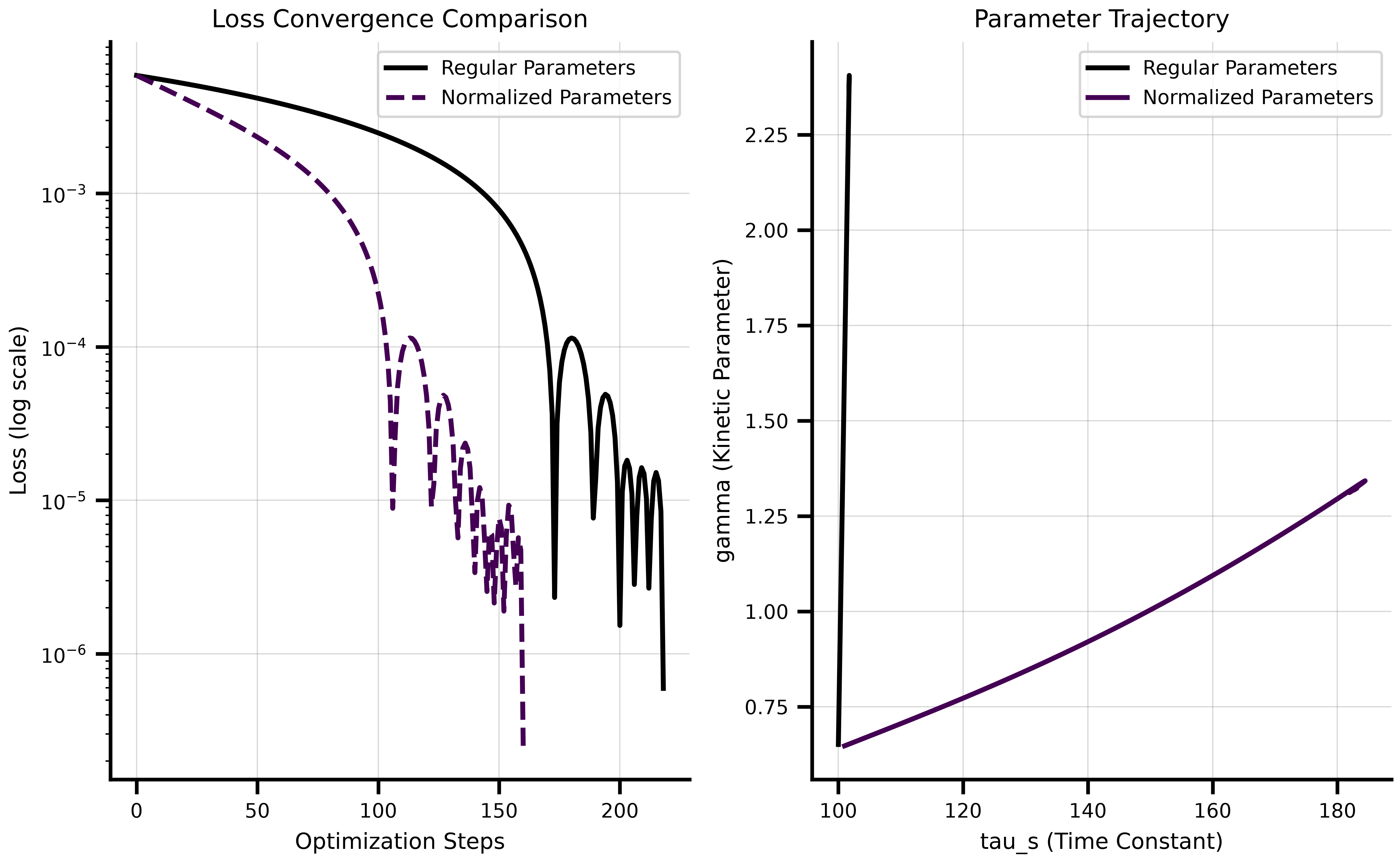
## Comparing Optimization Performance
The normalized parameters converge faster than regular parameters. With regular `Parameter` objects alone, most of the optimization change was applied to `gamma` while `tau_s` barely changed due to scaling differences and a learning rate of 0.01.
### Visualization of Convergence
The plots below show the optimization convergence and the parameter trajectories:
```{python}
#| code-fold: true
#| code-summary: "Show visualization code"
import matplotlib.pyplot as plt

fig, (ax1, ax2) = plt.subplots(1, 2, figsize=(8.1, 5.0625))

# Loss convergence comparison
ax1.semilogy(fitting_data["loss"].save, label='Regular Parameters', linewidth=2)
ax1.semilogy(fitting_data_norm["loss"].save, label='Normalized Parameters', linewidth=2, linestyle='--')
ax1.set_xlabel('Optimization Steps')
ax1.set_ylabel('Loss (log scale)')
ax1.set_title('Loss Convergence Comparison')
ax1.legend()
ax1.grid(True, alpha=0.3)

# Parameter trajectory in 2D space
gamma_traj = collect_parameters([p.gamma for p in fitting_data["parameters"].save])
tau_s_traj = collect_parameters([p.tau_s for p in fitting_data["parameters"].save])
gamma_traj_norm = collect_parameters([p.gamma for p in fitting_data_norm["parameters"].save])
tau_s_traj_norm = collect_parameters([p.tau_s for p in fitting_data_norm["parameters"].save])

ax2.plot(tau_s_traj, gamma_traj, label='Regular Parameters', linewidth=2)
ax2.plot(tau_s_traj_norm, gamma_traj_norm, label='Normalized Parameters', linewidth=2)
ax2.set_xlabel('tau_s (Time Constant)')
ax2.set_ylabel('gamma (Kinetic Parameter)')
ax2.set_title('Parameter Trajectory')
ax2.legend()
ax2.grid(True, alpha=0.3)

plt.tight_layout()
plt.show()
```
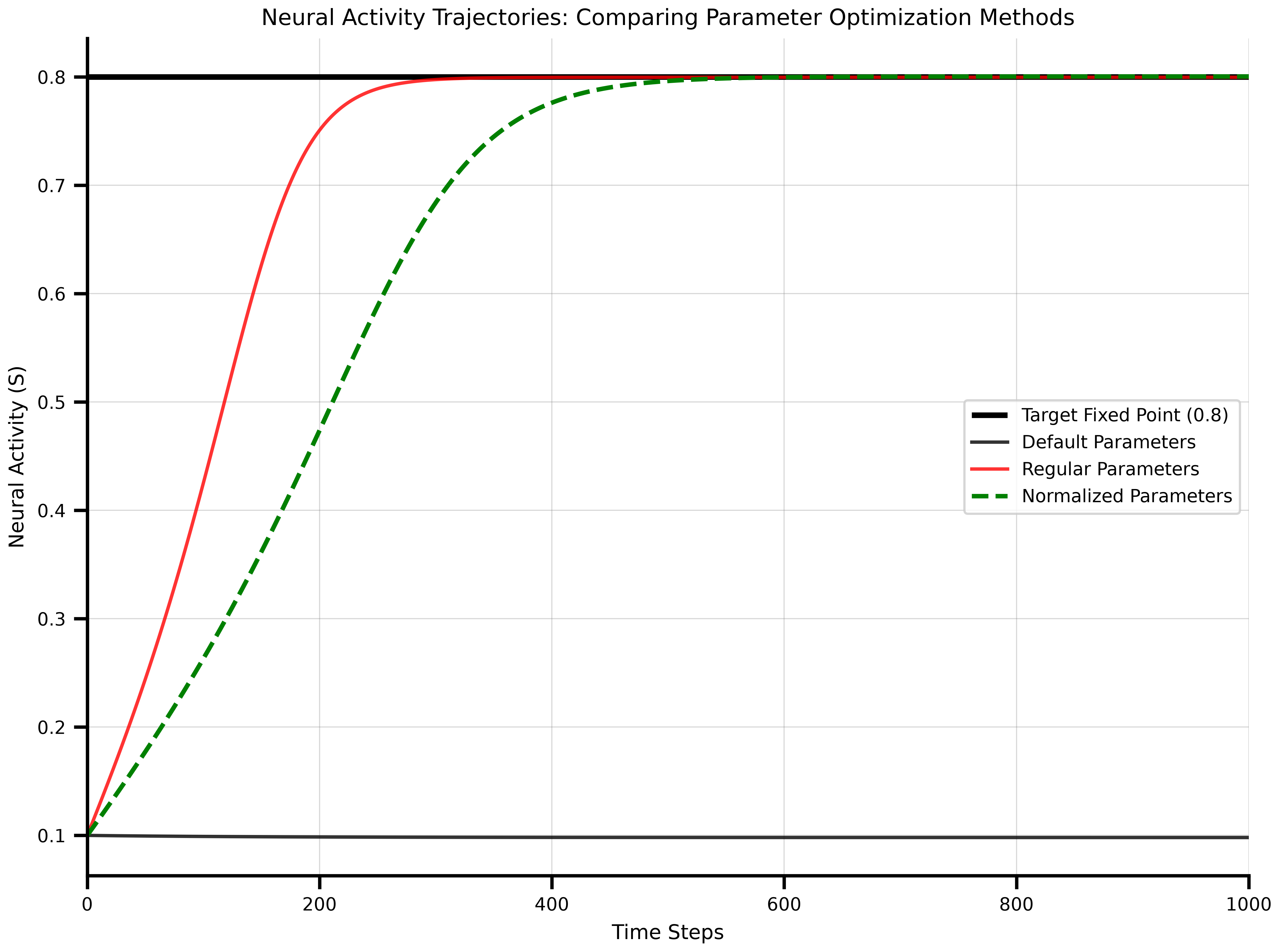
### Validating the Fixed Point Solution
Finally, run simulations with the optimized parameters to verify they reach the target fixed point at 0.8:
```{python}
# Run simulation with default parameters
m = ReducedWongWang()
ts_default = m.simulate(t1 = 1000, dt = 1.0)

# Run simulation with optimized parameters (regular Parameter)
p_opt = collect_parameters(p_opt)
m = ReducedWongWang(gamma = p_opt.gamma, tau_s = p_opt.tau_s)
ts_opt = m.simulate(t1 = 1000, dt = 1.0)

# Run simulation with optimized normalized parameters
p_opt_norm = collect_parameters(p_opt_norm)
m = ReducedWongWang(gamma = p_opt_norm.gamma, tau_s = p_opt_norm.tau_s)
ts_opt_norm = m.simulate(t1 = 1000, dt = 1.0)
```
The plot below shows how well each optimization approach reached the target fixed point:
```{python}
#| code-fold: true
#| code-summary: "Show visualization code"
fig, ax = plt.subplots(figsize=(8.1, 6.075))

# Plot target line
ax.hlines(0.8, 0, 1000, color="black", linewidth=2.5, label="Target Fixed Point (0.8)")

# Plot time series
ax.plot(ts_default[1][:, 0, :], label="Default Parameters", alpha=0.8)
ax.plot(ts_opt[1][:, 0, :], color='red', label="Regular Parameters", alpha=0.8)
ax.plot(ts_opt_norm[1][:, 0, :], color='green', linestyle='--',
        label="Normalized Parameters", linewidth=2)

ax.set_xlabel('Time Steps')
ax.set_ylabel('Neural Activity (S)')
ax.set_title('Neural Activity Trajectories: Comparing Parameter Optimization Methods')
ax.legend(loc="right")
ax.grid(True, alpha=0.3)
ax.set_xlim(0, 1000)
plt.tight_layout()
plt.show()
```
Both optimized parameter sets settle at the target 0.8, while the default parameters equilibrate elsewhere.