---
title: "Network Dynamics"
format:
html:
code-fold: false
toc: true
echo: true
fig-width: 8
out-width: "100%"
jupyter: python3
execute:
cache: true
---
::: {.callout-warning title="Experimental Feature"}
The interface to design network dynamics is still under development and might change in future releases.
:::
# What is Network Dynamics?
Network Dynamics is a pure JAX interface for defining and simulating brain network models. If you're familiar with TVB (The Virtual Brain), you'll recognize the core concepts, dynamics models, structural connectivity, coupling functions, and numerical integration. The key difference is that Network Dynamics is built entirely on JAX, making it:
- **Differentiable**: Gradients flow through the entire simulation for parameter optimization
- **JIT-compilable**: Automatic compilation for high-performance execution
- **GPU-ready**: Support for GPU acceleration
- **Explicit**: Clear separation of concerns with minimal magic
This document provides a gentle introduction through a complete working example, comparing the traditional TVB approach with the Network Dynamics framework. For detailed documentation on each component, see the linked sections throughout.
# A Complete Example: TVB vs Network Dynamics
Let's simulate a resting-state brain network using the Reduced Wong-Wang model with empirical connectivity. We'll show both approaches side-by-side so you can see the correspondence between frameworks.
::: {.callout-note collapse="true"}
## Mathematical Framework
Network Dynamics implements TVB's standard mathematical framework for brain network simulations. While this framework is the default, Network Dynamics can in principle model other system architectures due to its flexible JAX-based design.
The standard TVB framework simulates systems of stochastic differential equations with the following structure:
$$
\begin{align*}
dS_i &= \left[f_d(S_i, \theta^d, C_i, I_i) \right]dt + g(S_i, \theta^g)\, dW_i \\
C_i &= f_c^{\text{post}}\left(\sum_j A_{ij}\, f_c^{\text{pre}}(S_i, S_j(t-\tau_{ij}), \theta^c), S_i, \theta^c\right)
\end{align*}
$$
**State Evolution** (first equation):
- $S_i$ - state variables at node $i$ (e.g., membrane potential, synaptic gating)
- $f_d$ - dynamics function defining local temporal evolution with parameters $\theta^d$
- $C_i$ - coupling input from connected nodes
- $I_i$ - external input (stimulation, driving signals)
- $g$ - diffusion coefficient controlling noise intensity with parameters $\theta^g$
- $dW_i$ - Wiener process (Brownian motion) for stochastic fluctuations
**Coupling** (second equation):
- $f_c^{\text{pre}}$ - pre-aggregation transformation (e.g., state differences, nonlinearities)
- $A_{ij}$ - structural connectivity weight from node $j$ to node $i$
- $\tau_{ij}$ - transmission delay from tract length and conduction speed
- $f_c^{\text{post}}$ - post-aggregation transformation (e.g., gain, offset)
- $\theta^c$ - coupling parameters (strength, thresholds, etc.)
Each code component in Network Dynamics directly implements one part of this mathematical structure, making the mapping from theory to implementation transparent.
:::
::: {.columns}
::: {.column width="48%"}
### TVB Framework
```{python}
#| code-fold: true
#| code-summary: "Imports"
import warnings
import numpy as np

with warnings.catch_warnings():
    warnings.simplefilter("ignore")
    from tvb.simulator.lab import (
        models, connectivity, coupling,
        integrators, monitors, simulator
    )

from tvboptim.data import (
    load_structural_connectivity
)
```
```{python}
# Load connectivity data
weights, lengths, labels = (
    load_structural_connectivity("dk_average")
)

# Normalize weights
weights = weights / np.max(weights)

# Create connectivity object
conn = connectivity.Connectivity(
    weights=np.array(weights),
    tract_lengths=np.array(lengths),
    region_labels=np.array(labels),
    centres = np.zeros(84),
    speed=np.array([3.0])
)

# Create dynamics (defaults used)
model = models.ReducedWongWang(
    w=np.array([0.7])
)


# Create coupling
coupl = coupling.Linear(
    a=np.array([0.5])
)

# Create noise
# Note: TVB uses nsig = 0.5 * sigma^2
# where sigma is the desired std
sigma = 0.01
sigma_tvb = 0.5 * sigma**2
integrator = integrators.HeunStochastic(
    dt=1.0,
    noise=integrators.noise.Additive(
        nsig=np.array([sigma_tvb])
    )
)

# Build simulator
sim = simulator.Simulator(
    model=model,
    connectivity=conn,
    coupling=coupl,
    integrator=integrator,
    initial_conditions=0.1 * np.ones((100,1,84,1)),
)

sim.configure()

# Run simulation
print("Running TVB...")
(time_tvb, data_tvb), = sim.run(
    simulation_length=1000.0
)

print(f"Shape: {data_tvb.shape}")
```
:::
::: {.column width="4%"}
:::
::: {.column width="48%"}
### Network Dynamics Framework
```{python}
#| code-fold: true
#| code-summary: "Imports"
import jax
import jax.numpy as jnp
from tvboptim.experimental.network_dynamics import (
    Network, solve
)
from tvboptim.experimental.network_dynamics.dynamics.tvb import (
    ReducedWongWang
)
from tvboptim.experimental.network_dynamics.coupling import (
    DelayedLinearCoupling
)
from tvboptim.experimental.network_dynamics.graph import (
    DenseDelayGraph
)
from tvboptim.experimental.network_dynamics.noise import (
    AdditiveNoise
)
from tvboptim.experimental.network_dynamics.solvers import (
    Heun
)
from tvboptim.data import (
    load_structural_connectivity
)
```
```{python}
# Load connectivity data
weights, lengths, labels = (
    load_structural_connectivity("dk_average")
)

# Normalize weights
weights = weights / jnp.max(weights)
# Compute delays from tract lengths
delays = lengths / 3.0

# Create graph (connectivity + delays)
graph = DenseDelayGraph(
    weights, delays, region_labels=labels
)


# Create dynamics (defaults used)
dynamics = ReducedWongWang(
    INITIAL_STATE=(0.1),
    w=0.7
)

# Create coupling
coupling = DelayedLinearCoupling(
    incoming_states='S', G=0.5
)

# Create noise
# Note: Network Dynamics uses sigma
# as the std of additive noise
noise = AdditiveNoise(
    sigma=0.01, key=jax.random.key(42)
)


# Build network
network = Network(
    dynamics=dynamics,
    coupling={"delayed": coupling},
    graph=graph,
    noise=noise
)

# Create solver
solver = Heun()

# Run simulation
print("Running Network Dynamics...")
result = solve(
    network, solver,
    t0=0.0, t1=1000.0, dt=1.0
)

print(f"Shape: {result.ys.shape}")
```
:::
:::
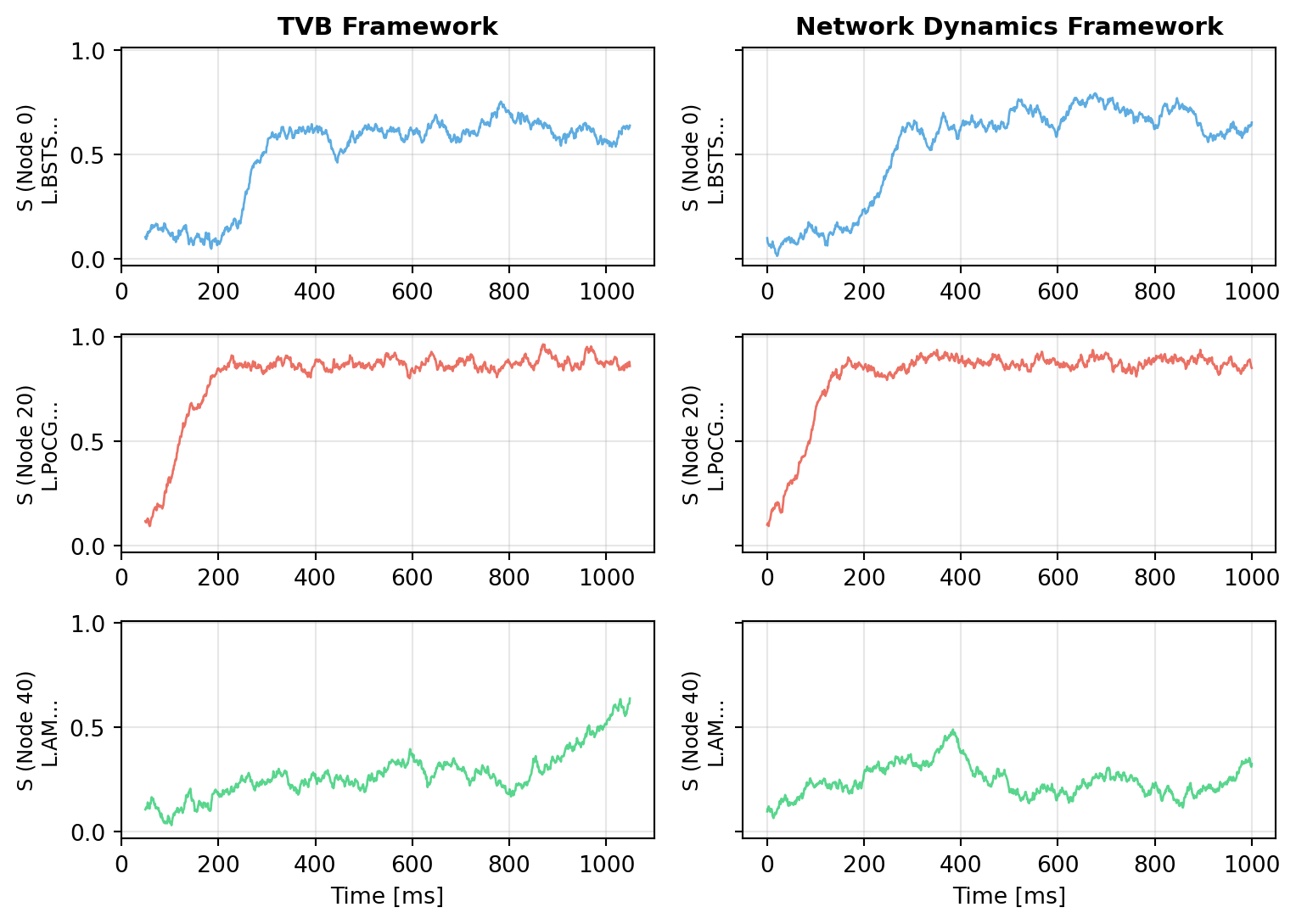
## Comparing the Results
Let's visualize both simulations to verify they produce comparable dynamics:
```{python}
#| code-fold: true
#| code-summary: "Visualization Code"
import matplotlib.pyplot as plt

fig, axes = plt.subplots(3, 2, figsize=(8.1, 5.786), sharey=True)

# Select a few representative nodes
nodes_to_plot = [0, 20, 40]
colors = ['#3498db', '#e74c3c', '#2ecc71']

# Time series comparison
for idx, node in enumerate(nodes_to_plot):
    # TVB result
    axes[idx, 0].plot(time_tvb - 50, data_tvb[:, 0, node, 0],
                      color=colors[idx], linewidth=1, alpha=0.8)
    axes[idx, 0].set_ylabel(f'S (Node {node})\n{labels[node][:15]}...', fontsize=9)
    axes[idx, 0].grid(True, alpha=0.3)
    if idx == 0:
        axes[idx, 0].set_title('TVB Framework', fontweight='bold', fontsize=11)
    if idx == len(nodes_to_plot) - 1:
        axes[idx, 0].set_xlabel('Time [ms]')

    # Network Dynamics result
    axes[idx, 1].plot(result.ts, result.ys[:, 0, node],
                      color=colors[idx], linewidth=1, alpha=0.8)
    axes[idx, 1].set_ylabel(f'S (Node {node})\n{labels[node][:15]}...', fontsize=9)
    axes[idx, 1].grid(True, alpha=0.3)
    if idx == 0:
        axes[idx, 1].set_title('Network Dynamics Framework', fontweight='bold', fontsize=11)
    if idx == len(nodes_to_plot) - 1:
        axes[idx, 1].set_xlabel('Time [ms]')

plt.tight_layout()
plt.show()
```
The time series show qualitatively similar dynamics - both frameworks produce realistic resting-state activity with fluctuations around the fixed point, driven by noise and network interactions. The differences come from different noise realizations in numpy (TVB) and JAX (Network Dynamics).
::: {.callout-important title="Noise Parameter Difference"}
**TVB** and **Network Dynamics** use different noise parameterizations:
- **TVB**: The `nsig` parameter in `integrators.noise.Additive()` is set as `nsig = 0.5 * sigma^2`, where `sigma` is the desired standard deviation. This is **not** the variance (which would be `sigma^2`), but a scaled version specific to TVB's implementation.
- **Network Dynamics**: The `sigma` parameter in `AdditiveNoise()` directly represents the **standard deviation** of the additive Gaussian noise.
To match noise levels between frameworks, use the conversion: `nsig_tvb = 0.5 * sigma_network^2`
:::
# Component Breakdown
The Network Dynamics framework consists of several modular components that work together. Each component implements a specific part of the mathematical structure described above.
## Dynamics
**Implements**: $f_d(S_i, \theta^d, C_i, I_i)$ - the local temporal evolution function
The **dynamics** define the differential equations at each network node, these are your neural mass models, oscillators, or other dynamical systems.
```python
dynamics = ReducedWongWang(w=0.7) # w is a parameter in θ^d
```
All TVB models are available out of the box and validated for Network Dynamics.
**→ See [Dynamics](dynamics.qmd) for details on models and creating custom dynamics**
## Graph (Connectivity)
**Implements**: $A_{ij}$ and $\tau_{ij}$ - the structural connectivity and transmission delays
The **graph** encodes the structural connectivity between nodes, which regions connect to which, with what strength, and with what delays.
```python
graph = DenseDelayGraph(weights, lengths, region_labels=labels)
```
Supports both dense and sparse representations, with optional transmission delays computed from tract lengths.
**→ See [Graph](graph.qmd) for connectivity representations and empirical datasets**
## Coupling
**Implements**: $f_c^{\text{pre}}$, $f_c^{\text{post}}$, and the summation $\sum_j A_{ij}\, f_c^{\text{pre}}(\cdots)$
The **coupling** defines how nodes interact through the connectivity, this transforms states from connected nodes into input to the local dynamics.
```python
coupling = DelayedLinearCoupling(incoming_states='S', G=0.5) # G is part of θ^c
```
The coupling pattern mirrors TVB's pre-sum-post architecture. You can use instantaneous or delayed coupling, linear or nonlinear transformations.
**→ See [Coupling](coupling.qmd) for coupling types, delays, and custom implementations**
## Noise (Optional)
**Implements**: $g(S_i, \theta^g)$ - the diffusion coefficient controlling noise intensity
The **noise** component adds stochastic fluctuations to the dynamics, transforming ODEs into SDEs.
```python
noise = AdditiveNoise(sigma=0.01, key=jax.random.key(42)) # sigma is θ^g
```
Supports additive and multiplicative noise, with selective application to specific state variables. The Wiener process $dW_i$ is automatically handled by the solver.
**→ See [Noise](noise.qmd) for stochastic processes and noise types**
## External Inputs (Optional)
**Implements**: $I_i$ - external driving signals from outside the network
The **external input** system provides time-dependent (or state-dependent) driving signals from outside the network.
```python
external_input = DataInput(times, data, interpolation='cubic')
```
Use parametric inputs (sine waves, pulses) or data-based inputs (interpolated recordings).
**→ See [External Inputs](external_inputs.qmd) for stimulation and driving signals**
## Solvers
**Implements**: Numerical integration of $dS_i = [\cdots]dt + g\,dW_i$
The **solver** performs numerical integration of the network dynamics using various methods (Euler, Heun, Runge-Kutta).
```python
solver = Heun()
result = solve(network, solver, t0=0.0, t1=1000.0, dt=0.5)
```
Native solvers (Euler, Heun, RK4) are optimized for brain networks and support all features. Diffrax solvers provide advanced methods for special cases.
**→ See [Solvers](solvers.qmd) for integration methods and performance considerations**
# Design Philosophy
Network Dynamics is built on a few core principles that shape its architecture and user experience:
## Pure JAX Foundation
Everything is JAX from the ground up:
- **Differentiable**: Automatic gradients through entire simulations enable gradient-based parameter optimization
- **JIT-compiled**: Automatic compilation to optimized machine code (CPU/GPU/TPU)
- **Vectorizable**: `vmap` for efficient batch simulations across parameter sets or initial conditions
- **GPU-ready**: Seamless acceleration on GPUs without code changes
## Explicit Over Implicit
Every operation is visible and controllable:
- **No hidden state**: All parameters, initial conditions, and configurations are explicitly provided
- **Clear data flow**: Function signatures show exactly what goes in and what comes out
- **Transparent components**: Each component (dynamics, coupling, noise) has a simple, documented interface
- **No magic**: What you write is what executes, no automatic configuration or hidden transformations
## Composability
Mix and match components freely:
- **Modular design**: Swap dynamics models, coupling functions, or solvers without changing other parts, similar to TVB
- **Custom components**: Subclass base classes to implement novel dynamics, coupling, or noise
- **Multiple couplings**: Combine instantaneous and delayed, linear and nonlinear coupling in a single network
- **Flexible noise**: Apply noise selectively to specific state variables
## Optimization-First Design
Built for parameter inference and model fitting through a pure functional architecture:
**The `prepare()` pattern**: Under the hood, `solve()` calls `prepare()` which separates state from execution:
```python
# High-level: convenient class-based API
result = solve(network, solver, t0=0.0, t1=1000.0, dt=0.5)

# Under the hood: prepare() returns a pure function and state
solve_fn, state = prepare(network, solver, t0=0.0, t1=1000.0, dt=0.5)
result = solve_fn(state)  # Pure function call with PyTree state
```
**Why this enables optimization**:
- The `Network`, `Dynamics`, `Coupling` classes are convenient builders for complex parameter structures
- `prepare()` compiles everything into a pure function and a PyTree of parameters
- This pure function can be passed to JAX transformations: `jit`, `grad`, `vmap`
- Direct gradient access: Use JAX's `grad()` or `value_and_grad()` on `solve_fn`
- The state is just nested dictionaries (Bunch objects), fully compatible with JAX's PyTree system
- Mark parameters for optimization with `Parameter` and `BoundedParameter`
- Easy integration with Optax, BlackJAX, and other JAX optimization libraries
- Efficiently explore parameter spaces with `vmap` for batch simulations
- Inspect, modify, or serialize the state as plain data
This architecture gives you the convenience of high-level classes while maintaining JAX's functional core for optimization.
# Key Differences from TVB
If you're coming from TVB, here are the main architectural differences:
## Observations & Monitoring
**TVB approach**: Monitors sample the simulation during integration, selecting variables and applying transformations (downsampling, BOLD, etc.) in real-time.
**Network Dynamics approach**: Simulations return the full time series, and observations are applied as post-processing. TVB-compatible observation functions are available in `tvboptim.observations.tvb_monitors`:
```python
from tvboptim.observations.tvb_monitors import Bold, SubSampling

# Run simulation - get full time series
result = solve(network, solver, t0=0.0, t1=10000.0, dt=1.0)

# Create BOLD monitor with standard parameters
bold_monitor = Bold(
    period=720.0,           # BOLD sampling period (1 TR = 720 ms)
    downsample_period=4.0,  # Intermediate downsampling matches dt
    voi=0,                  # Monitor first state variable (S)
)

# Create subsampling monitor with standard parameters
downsampling_monitor = SubSampling(
    period=10.0,  # Subsample period (10 ms)
)

# Apply observations as post-processing
bold_signal = bold_monitor(result)
downsampled = downsampling_monitor(result)
```
This makes the pipeline more transparent, you can inspect the raw simulation output, apply different observations to the same data, and compose observation functions.
## No Modes Dimension
**TVB**: Output has shape `[time, state, nodes, modes]` where modes represent different oscillation modes or population types.
**Network Dynamics**: Output has shape `[time, state, nodes]`. If your model has multiple populations (e.g., excitatory/inhibitory), these are represented as separate state variables.
This simplifies indexing and makes it clearer what each dimension represents.
## Noise Parameterization
As noted earlier, noise parameters differ:
- **TVB**: `nsig = 0.5 * sigma^2` (scaled parameter specific to TVB's implementation)
- **Network Dynamics**: `sigma` directly represents the standard deviation of Gaussian noise or `sigma = $\sqrt{2\ \mathrm{nsig}}$`
The Network Dynamics parameterization is more intuitive and matches standard SDE literature.
# Next Steps
## Start Exploring Components
Depending on your use case, dive into the detailed documentation:
1. **Want to understand dynamics models?** → Start with [Dynamics](dynamics.qmd) to see available models and create custom ones
2. **Working with custom connectivity?** → Check [Graph](graph.qmd) for dense/sparse representations and empirical datasets
3. **Need specialized coupling?** → See [Coupling](coupling.qmd) for coupling types, delays, and performance considerations
4. **Adding stochasticity?** → Explore [Noise](noise.qmd) for additive and multiplicative processes
5. **Stimulating the network?** → Read [External Inputs](external_inputs.qmd) for parametric and data-based stimulation
6. **Optimizing performance?** → Study [Solvers](solvers.qmd) for native vs Diffrax methods
## Complete Optimization Workflows
Ready to see the full power of Network Dynamics? These end-to-end tutorials demonstrate complete parameter optimization workflows, from setting up networks to fitting model parameters to empirical data using gradient-based optimization:
### [Reduced Wong-Wang FC Optimization(RWW)](../workflows/RWW.qmd)
Learn how to fit a whole-brain resting-state network model to empirical fMRI functional connectivity. This tutorial covers:
- Setting up the RWW dynamics with structural connectivity
- Defining loss functions for FC fitting
- Exploring parameter sensitivity
### [Jansen-Rit MEG Peak Frequency Gradient Optimization (JR)](../workflows/JR.qmd)
Reproduce the spatial frequency gradient observed in resting-state MEG data, where peak frequencies vary from ~7 Hz in association areas to ~11 Hz in sensory cortex. This tutorial demonstrates:
- Modeling cortical columns with the Jansen-Rit neural mass model
- Parameter exploration using grid search to map the frequency landscape
- Defining region-specific optimization targets from neuroimaging data
- Fitting heterogeneous (region-specific) parameters with gradient-based optimization
- Spectral analysis and validation against empirical patterns
## Get Help
- Check the [API Reference](../reference/index.qmd) for detailed parameter descriptions
- Look at examples in the repository
- Report issues or ask questions on GitHub