---
title: "Define a Brain Network Model in TVB-Optim, TVB-O, or TVB"
description: "This page provides installation instructions and guides you through the TVB-Optim workflow. We follow a parallel structure depending on how you want to define your brain network model."
format:
html:
code-fold: false
toc: true
echo: false
fig-width: 8
out-width: "100%"
code-tools:
source: true
toggle: true
code-download: true
jupyter: python3
execute:
cache: true
---
## Installation & Requirements
TVB-Optim requires Python 3.11 or later and depends on JAX for high-performance computing and automatic differentiation.
### Install TVB-Optim
TVB-Optim is a standalone package that provides utilities for optimization algorithms, parameter spaces, and execution strategies. You can define models directly in TVB-Optim or use models from other frameworks:
::: {.panel-tabset}
## UV
```bash
uv pip install tvboptim
```
For development:
```bash
git clone https://github.com/virtual-twin/tvboptim.git
cd tvboptim
uv pip install -e ".[dev]"
```
## pip
```bash
pip install tvboptim
```
For development:
```bash
git clone https://github.com/virtual-twin/tvboptim.git
cd tvboptim
pip install -e ".[dev]"
```
:::
### Optional: Install TVB-O
TVB-O is **only required** if you want to:
- Use models defined in classic TVB (The Virtual Brain)
- Access models from the TVB ontology
- Utilize pre-defined brain connectivity data and atlases
If you need TVB-O, install it with:
::: {.panel-tabset}
## UV
```bash
uv pip install tvbo
```
For development:
```bash
git clone https://github.com/virtual-twin/tvbo.git
cd tvboptim
uv pip install -e ".[dev]"
```
## pip
```bash
pip install tvbo
```
For development:
```bash
git clone https://github.com/virtual-twin/tvbo.git
cd tvboptim
pip install -e ".[dev]"
```
:::
```{python}
#| output: false
#| code-fold: true
#| code-summary: "Imports"
#| echo: true
# Set up environment
import os
import time
import copy

# Mock devices to force JAX to parallelize on CPU (pmap trick)
# This allows parallel execution even without multiple GPUs
cpu = True
if cpu:
    N = 8  # Number of virtual devices to create
    os.environ['XLA_FLAGS'] = f'--xla_force_host_platform_device_count={N}'

# Import all required libraries
from scipy import io
import numpy as np
import matplotlib.pyplot as plt
import jax
import jax.numpy as jnp
import copy
import optax  # JAX-based optimization library
from IPython.display import Markdown

# Import from tvboptim - our optimization and execution framework
from tvboptim import prepare  # Converts TVB-O experiments to JAX functions
from tvboptim.types import Parameter  # Parameter types
from tvboptim.types.spaces import Space, GridAxis  # Parameter spaces
from tvboptim.types.stateutils import show_parameters  # Utility functions
from tvboptim.utils import set_cache_path, cache  # Caching for expensive computations
# from tvboptim.observations import   # Observation functions (FC, RMSE, etc.)
from tvboptim.execution import ParallelExecution, SequentialExecution  # Execution strategies
from tvboptim.optim.optax import OptaxOptimizer  # JAX-based optimizer with automatic differentiation
from tvboptim.optim.callbacks import MultiCallback, DefaultPrintCallback, StopLossCallback  # Optimization callbacks

# Import network_dynamics from tvboptim.experimental - for standalone TVB-Optim models
from tvboptim.experimental import network_dynamics as nd
from tvboptim.experimental.network_dynamics.dynamics import ReducedWongWang
from tvboptim.experimental.network_dynamics.coupling import LinearCoupling
from tvboptim.experimental.network_dynamics.graph import DenseDelayGraph
from tvboptim.experimental.network_dynamics.solvers import Heun
from tvboptim.experimental.network_dynamics.noise import AdditiveNoise
from tvboptim.data import load_structural_connectivity

# Import from tvbo - the brain simulation framework
from tvbo import SimulationExperiment  # Main experiment class
from tvbo.datamodel import tvbo_datamodel  # Data structures
from tvbo.utils import numbered_print  # Utility functions

# Classic TVB imports - for using TVB simulator directly
import warnings
with warnings.catch_warnings():
    warnings.simplefilter("ignore")
    from tvb.simulator.lab import simulator, models, connectivity, coupling, integrators, monitors

# Set cache path for tvboptim - stores expensive computations for reuse
set_cache_path("./get_started")
```
```{python}
#| output: false
#| code-fold: true
#| code-summary: "Load Data"
#| echo: true
# Load structural connectivity data from Desikan-Killiany atlas
# Returns: weights (connectivity matrix), lengths (tract lengths in mm), labels (region names)
weights, lengths, labels = load_structural_connectivity("dk_average")

# Normalize weights to [0, 1] range
weights = weights / np.max(weights)

# Calculate delays from tract lengths and conduction speed (3 mm/ms)
speed = np.inf
delays = lengths / speed
```
## Create a Brain Network Model
::: {.panel-tabset}
## TVB-Optim
```{python}
#| echo: true
# Define the local dynamics for each node: Reduced Wong-Wang model
# w: excitatory recurrence strength, I_o: external input, INITIAL_STATE: starting condition
dynamics = ReducedWongWang(w=0.5, I_o=0.32, INITIAL_STATE=(0.3,))
# Define coupling between nodes: Linear coupling
# incoming_states: which state variable to couple, G: global coupling strength
coup = LinearCoupling(incoming_states='S', G=0.75)
# Define the network structure: connectivity weights and delays
graph = DenseDelayGraph(weights, delays)
# Add noise to the system: additive noise applied to state variable S
noise = AdditiveNoise(sigma=0.002, apply_to="S", key=jax.random.key(42))
# Create the network by combining all components
# The coupling is labeled "delayed" (vs "instant" for instantaneous coupling)
network = nd.Network(dynamics, {"delayed": coup}, graph, noise=noise)
# Solve the network dynamics using Heun stochastic integrator
# t0=0, t1=10000 (ms), dt=4.0 (integration step size in ms)
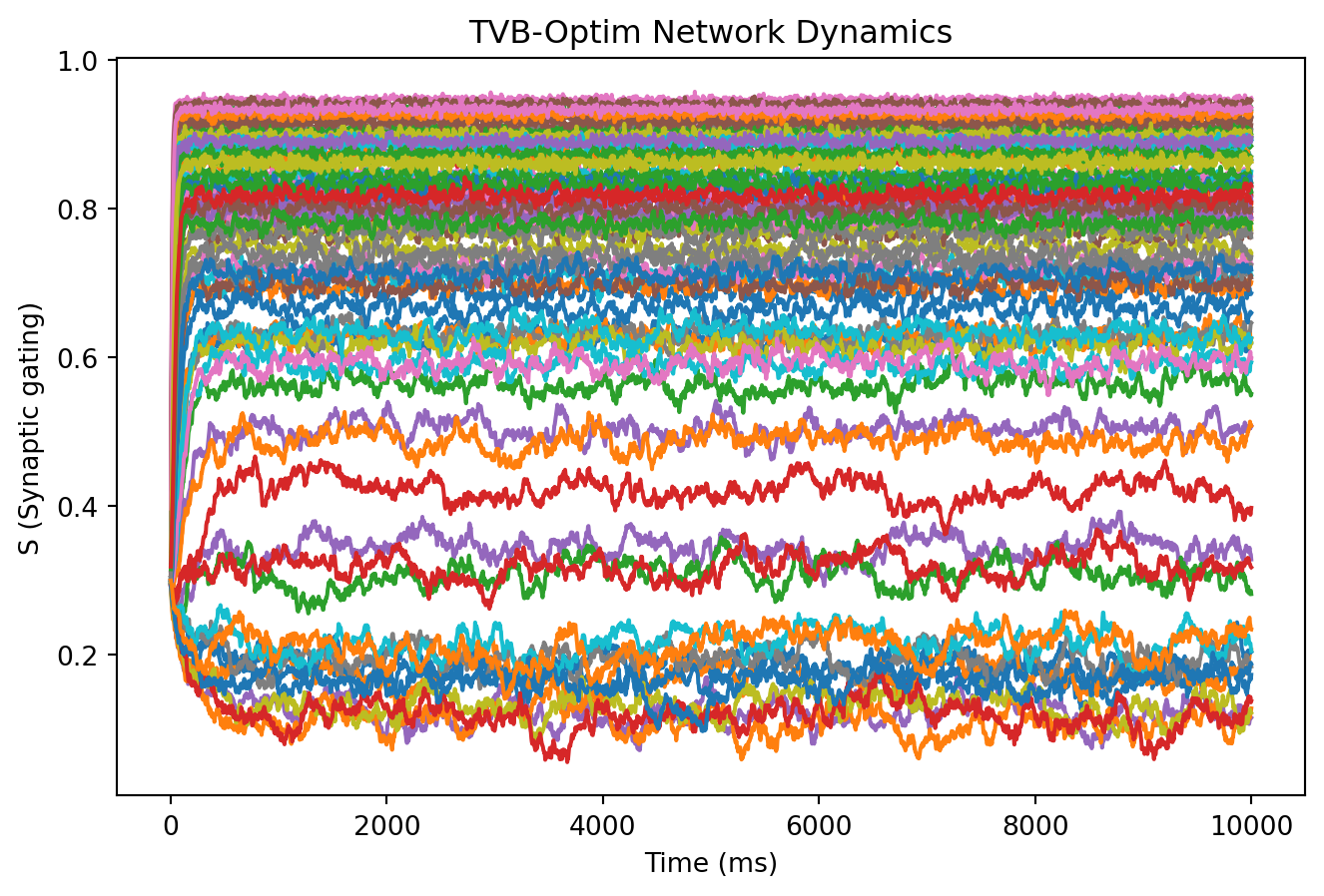
result = nd.solve(network, Heun(), t0=0, t1=10_000, dt=4.0)
# Plot time series: all regions (columns) over time (rows)
plt.plot(result.ts, result.ys[:, 0, :])
plt.xlabel("Time (ms)")
plt.ylabel("S (Synaptic gating)")
plt.title("TVB-Optim Network Dynamics");
```
## TVB-O
For all the details on TVB-O, see its [Documentation](https://virtual-twin.github.io/tvbo). A simple experiment can be created like this:
```{python}
#| echo: true
#| eval: false
#| output: true
# Create a brain simulation experiment using the Reduced Wong-Wang model
# TVB-O uses a declarative dictionary-based approach
experiment = SimulationExperiment(
    model={
        "name": "ReducedWongWang",
        "parameters": {
            "w": {"name": "w", "value": 0.5},      # Excitatory recurrence strength
            "I_o": {"name": "I_o", "value": 0.32}, # External input current
        },
        "state_variables": {
            "S": {"initial_value": 0.3},  # Initial synaptic gating variable
        }
    },
    connectivity={
        "conduction_speed": {"name": "cs", "value": np.array([speed])}  # 3 mm/ms
    },
    coupling={
        "name": "Linear",
        "parameters": {"a": {"name": "a", "value": 0.75}}  # Global coupling strength
    },
    integration={
        "method": "Heun",        # Stochastic Heun integration
        "step_size": 4.0,        # Integration step in ms
        "noise": {"parameters": {"sigma": {"value": 0.002}}},  # Noise amplitude
        "duration": 10_000       # Total simulation time in ms
    },
    monitors={
        "Raw": {"name": "Raw"},  # Monitor raw state variables
    },
)

# Set the connectivity data loaded earlier
experiment.connectivity.weights = weights
experiment.connectivity.lengths = lengths
experiment.connectivity.metadata.number_of_regions = weights.shape[0]

# Configure the experiment (validates and prepares for simulation)
experiment.configure()

# Run the simulation and get results
result_tvbo = experiment.run(format="jax")

# Plot time series: all regions over time
plt.plot(result_tvbo.time, result_tvbo.data[:, 0, :, 0])
plt.xlabel("Time (ms)")
plt.ylabel("S (Synaptic gating)")
plt.title("TVB-O Experiment Results");
```
::: {.callout-note collapse="true" title="Create a Model Report"}
```{python}
#| eval: false
#| echo: true
Markdown(experiment.model.generate_report())
```
:::
::: {.callout-note collapse="true" title="You can inspect the rendered JAX code"}
```{python}
#| eval: false
#| echo: true
numbered_print(experiment.render_code(format = "jax"))
```
:::
## TVB
Classic simulator definition in TVB:
```{python}
#| eval: false
#| echo: true
# Define simulator using classic TVB (object-oriented approach)
sim = simulator.Simulator(
    # Model with parameters as numpy arrays
    model=models.ReducedWongWang(
        w=np.array([0.5]),      # Excitatory recurrence
        I_o=np.array([0.32])    # External input
    ),
    # Connectivity object with structural data
    connectivity=connectivity.Connectivity(
        weights=np.array(weights),
        tract_lengths=np.array(lengths),
        region_labels=np.array(labels),
        centres=np.zeros(weights.shape[0]),  # Dummy spatial coordinates
    ),
    # Linear coupling function
    coupling=coupling.Linear(a=np.array([0.75])),
    # Stochastic Heun integrator with additive noise
    integrator=integrators.HeunStochastic(
        noise=integrators.noise.Additive(nsig=np.array([0.5 * 0.002**2])),
        dt=4.0
    ),
    # Initial conditions: shape (history_length, state_vars, regions, modes)
    initial_conditions=0.3 * np.ones((50, 1, 84, 1)),
    simulation_length=10_000,  # Total time in ms
    monitors=(monitors.Raw(),)  # Record raw state variables
)

# Configure the simulator (sets up internal structures)
sim.configure()

# Convert classic TVB simulator to TVB-O experiment format
experiment_tvb = SimulationExperiment.from_tvb_simulator(sim)

# Run using JAX backend
result_tvb = experiment_tvb.run(format="jax")

# Plot time series: all regions over time
plt.plot(result_tvb.Raw.time, result_tvb.Raw.data[:, 0, :, 0])
plt.xlabel("Time (ms)")
plt.ylabel("S (Synaptic gating)")
plt.title("Classic TVB Simulator Results");
```
:::
## Get Model and State
::: {.panel-tabset}
## TVB-Optim
The `prepare` function separates network setup from execution, returning a pure function for simulation:
```{python}
#| echo: true
# Prepare the network for simulation - returns (model_fn, config)
# This separates setup from execution for better performance and composability
model, state = nd.prepare(network, Heun(), t0=0, t1=10_000, dt=4.0)
```
The `model` is a pure JAX function that takes the config and runs the simulation. The `state` contains all parameters, initial conditions, and precomputed data needed for the simulation.
## TVB-O
The `prepare` function converts the TVB-O experiment into a JAX-compatible model function and state object:
```{python}
#| eval: false
#| echo: true
# Convert TVB-O experiment to JAX function and state
model_tvbo, state_tvbo = prepare(experiment)
```
The `model` is a pure JAX function that takes the config and runs the simulation. The `state` contains all parameters, initial conditions, and precomputed data needed for the simulation.
:::
## Understand the State Object & Parameters
The state is of type `tvbo.utils.Bunch`, which is a `dict` with convenient get and set functions. At the same time, it is also a [`jax.Pytree`](https://docs.jax.dev/en/latest/pytrees.html), making it compatible with all of JAX's transformations. You can think of it as a big tree holding all parameters and initial conditions that uniquely define a simulation:
::: {.panel-tabset}
## TVB-Optim
```{python}
#| echo: true
state.keys()
```
## TVB-O
```{python}
#| eval: false
#| echo: true
state_tvbo
```
:::
## Simulate the Model
To run a simulation, you can simply call the model.
::: {.panel-tabset}
## TVB-Optim
```{python}
#| echo: true
# Run the simulation - model returns result object
result = model(state)
```
```{python}
#| echo: true
#| code-fold: true
#| code-summary: "Visualization"
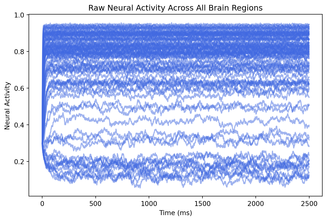
# Plot raw neural activity for all 84 brain regions over time
# Shape: [time_points, state_variables, regions]
plt.plot(result.data[:,0,:], color = "royalblue", alpha = 0.5)
plt.xlabel("Time (ms)")
plt.ylabel("Neural Activity")
plt.title("Raw Neural Activity Across All Brain Regions");
```
## TVB-O
```{python}
#| eval: false
#| echo: true
# Run the simulation - model returns (raw_activity, )
result = model_tvbo(state_tvbo)
raw = result[0]
```
```{python}
#| eval: false
#| echo: true
#| code-fold: true
#| code-summary: "Visualization"
# Plot raw neural activity for all 84 brain regions over time
# Shape: [time_points, state_variables, regions, modes]
plt.plot(raw.data[:,0,:,0], color = "royalblue", alpha = 0.5)
plt.xlabel("Time (ms)")
plt.ylabel("Neural Activity")
plt.title("Raw Neural Activity Across All Brain Regions");
```
:::
## Wrap the Model to create observations
We look at the mean activity of the last 500 timesteps as an easy observation.
::: {.panel-tabset}
## TVB-Optim
```{python}
#| echo: true
def observation(state):
    """
    Extract a simple observation from the simulation.
    We use the mean activity of the last 500 timesteps to avoid transient effects.
    """
    ts = model(state).data[-500:,0,:]  # Last 500 timesteps, skip transient
    mean_activity = jnp.mean(ts)  # Average across time and regions
    return mean_activity

# Test the observation function
print(f"Mean activity: {observation(state):.4f}")
```
## TVB-O
```{python}
#| echo: true
#| eval: false
def observation_tvbo(state):
    """
    Extract a simple observation from the simulation.
    We use the mean activity of the last 500 timesteps to avoid transient effects.
    """
    ts = model_tvbo(state)[0].data[-500:,0,:,0]  # Last 500 timesteps, skip transient
    mean_activity = jnp.mean(ts)  # Average across time and regions
    return mean_activity

# Test the observation function
print(f"Mean activity: {observation_tvbo(state_tvbo):.4f}")
```
:::
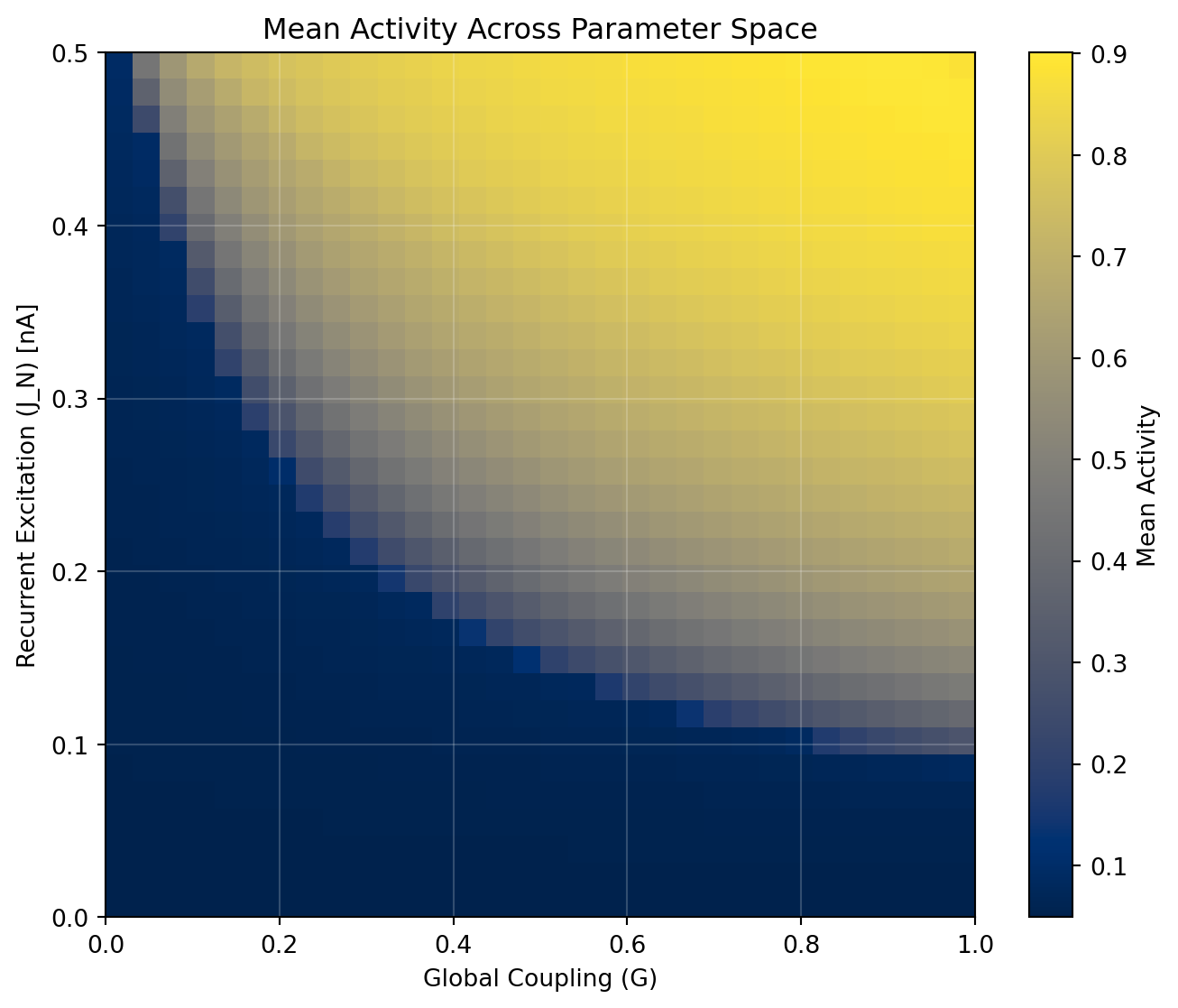
## Explore that across a parameter space
We can use a `Space` to explore how parameters `J_N` (excitatory recurrence) and `a` (global coupling) affect the observation. We use the cache decorator to save computationally demanding operations. We also parallelize the exploration using the `ParallelExecution` class with `n_pmap = 8`, which is possible because we told JAX that our CPU has 8 devices - known as the pmap trick.
::: {.panel-tabset}
## TVB-Optim
```{python}
#| echo: true
# Create a copy of the state for parameter exploration
exploration_state = copy.deepcopy(state)

# Set up parameter exploration by setting GridAxis in the state
n = 32  # 32x32 grid = 1024 parameter combinations
exploration_state.coupling.delayed.G = GridAxis(0.0, 1.0, n)
exploration_state.dynamics.J_N = GridAxis(0.0, 0.5, n)

# Create a grid space for systematic parameter exploration
params_space = Space(exploration_state, mode="product")

@cache("explore_tvboptim", redo = False)  # Cache results to avoid recomputation
def explore():
    # Use parallel execution with 8 virtual devices (pmap trick)
    exec = ParallelExecution(observation, params_space, n_pmap=8)
    return exec.run()

# Run the exploration (or load from cache)
exploration = explore()
```
```{python}
#| echo: true
#| code-fold: true
#| code-summary: "Visualization"
# Collect parameter values and results
coupling_vals = []
j_n_vals = []
activity_vals = []
for params, activity in zip(params_space, exploration):
    coupling_vals.append(params.coupling.delayed.G)
    j_n_vals.append(params.dynamics.J_N)
    activity_vals.append(activity)

# Convert to arrays
coupling_vals = jnp.array(coupling_vals)
j_n_vals = jnp.array(j_n_vals)
activity_vals = jnp.array(activity_vals)

# Create properly gridded heatmap
# Get unique sorted values for each parameter
unique_coupling = jnp.sort(jnp.unique(coupling_vals))
unique_j_n = jnp.sort(jnp.unique(j_n_vals))

# Create grid and map values
grid = jnp.zeros((len(unique_j_n), len(unique_coupling)))
for coupling, j_n, activity in zip(coupling_vals, j_n_vals, activity_vals):
    i = jnp.where(unique_j_n == j_n)[0][0]
    j = jnp.where(unique_coupling == coupling)[0][0]
    grid = grid.at[i, j].set(activity)

# Visualize the parameter space exploration
plt.figure(figsize=(8.1, 6.48))
im = plt.imshow(grid, aspect="auto", origin="lower",
                extent=[unique_coupling[0], unique_coupling[-1],
                       unique_j_n[0], unique_j_n[-1]],
                cmap="cividis")
plt.xlabel("Global Coupling (G)")
plt.ylabel("Recurrent Excitation (J_N) [nA]")
plt.title("Mean Activity Across Parameter Space")
plt.colorbar(im, label="Mean Activity")
plt.grid(True, alpha=0.2, color='white')
```
## TVB-O
```{python}
#| echo: true
#| eval: false
# Create a copy of the state for parameter exploration
exploration_state_tvbo = copy.deepcopy(state_tvbo)

# Set up parameter exploration by setting GridAxis in the state
n = 32  # 32x32 grid = 1024 parameter combinations
exploration_state_tvbo.parameters.coupling.a = GridAxis(0.0, 1.0, n)
exploration_state_tvbo.parameters.model.J_N = GridAxis(0.0, 0.5, n)

# Create a grid space for systematic parameter exploration
params_space_tvbo = Space(exploration_state_tvbo, mode="product")

@cache("explore_tvbo", redo = False)  # Cache results to avoid recomputation
def explore():
    # Use parallel execution with 8 virtual devices (pmap trick)
    exec = ParallelExecution(observation_tvbo, params_space_tvbo, n_pmap=8)
    return exec.run()

# Run the exploration (or load from cache)
exploration = explore()
```
```{python}
#| echo: true
#| code-fold: true
#| code-summary: "Visualization"
#| eval: false
# Collect parameter values and results
coupling_vals_tvbo = []
j_n_vals_tvbo = []
activity_vals_tvbo = []
for params, activity in zip(params_space_tvbo, exploration):
    coupling_vals_tvbo.append(params.parameters.coupling.a)
    j_n_vals_tvbo.append(params.parameters.model.J_N)
    activity_vals_tvbo.append(activity)

# Convert to arrays
coupling_vals_tvbo = jnp.array(coupling_vals_tvbo)
j_n_vals_tvbo = jnp.array(j_n_vals_tvbo)
activity_vals_tvbo = jnp.array(activity_vals_tvbo)

# Create properly gridded heatmap
# Get unique sorted values for each parameter
unique_coupling_tvbo = jnp.sort(jnp.unique(coupling_vals_tvbo))
unique_j_n_tvbo = jnp.sort(jnp.unique(j_n_vals_tvbo))

# Create grid and map values
grid_tvbo = jnp.zeros((len(unique_j_n_tvbo), len(unique_coupling_tvbo)))
for coupling, j_n, activity in zip(coupling_vals_tvbo, j_n_vals_tvbo, activity_vals_tvbo):
    i = jnp.where(unique_j_n_tvbo == j_n)[0][0]
    j = jnp.where(unique_coupling_tvbo == coupling)[0][0]
    grid_tvbo = grid_tvbo.at[i, j].set(activity)

# Visualize the parameter space exploration
plt.figure(figsize=(10, 8))
im = plt.imshow(grid_tvbo, aspect="auto", origin="lower",
                extent=[unique_coupling_tvbo[0], unique_coupling_tvbo[-1],
                       unique_j_n_tvbo[0], unique_j_n_tvbo[-1]],
                cmap="cividis")
plt.xlabel("Global Coupling (a)")
plt.ylabel("Recurrent Excitation (J_N) [nA]")
plt.title("Mean Activity Across Parameter Space")
plt.colorbar(im, label="Mean Activity")
plt.grid(True, alpha=0.2, color='white')
```
:::
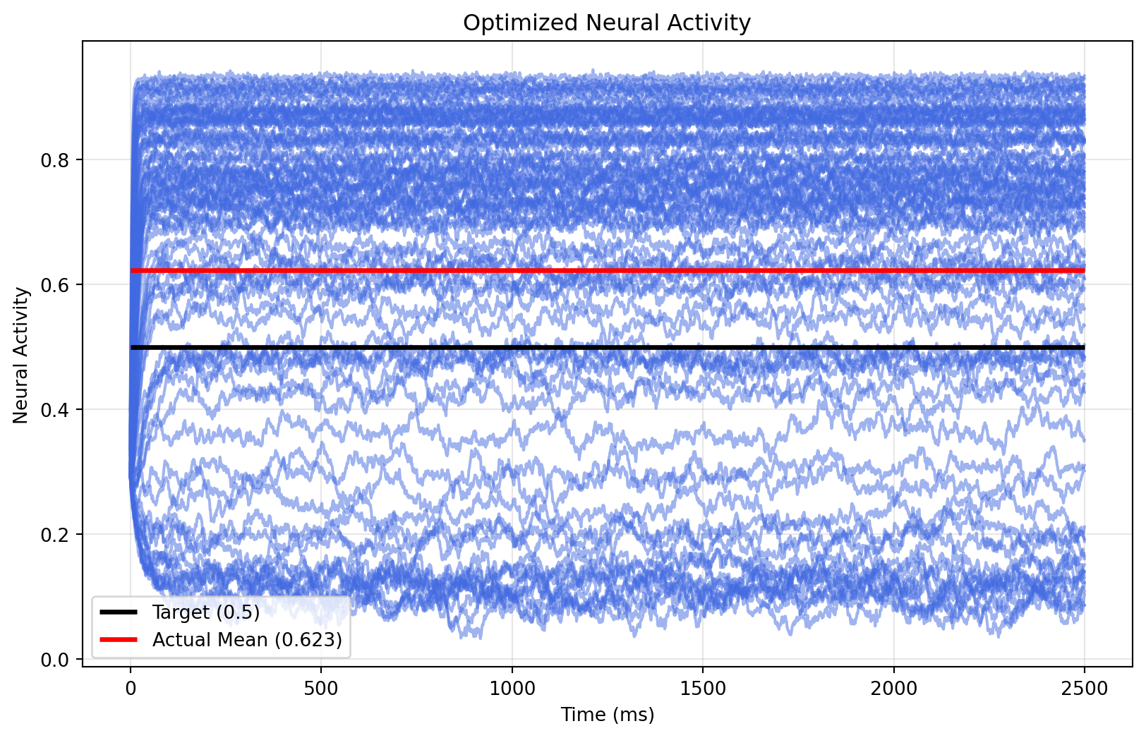
## Define a Loss and Optimize
Let's say our goal is to have a mean activity of 0.5. We can define a loss function that penalizes deviations from this target.
::: {.panel-tabset}
## TVB-Optim
```{python}
#| echo: true
def loss(state):
    """
    Define a loss function that penalizes deviations from target activity.
    Goal: Each brain region should have mean activity of 0.5
    """
    ts = model(state).data[-500:,0,:]  # Skip transient period
    mean_activity = jnp.mean(ts, axis = 0)  # Average over time for each region
    # Compute mean squared error between actual and target (0.5) activity
    return jnp.mean((mean_activity - 0.5)**2)  # Region-wise difference

# Test the loss function
print(f"Current loss: {loss(state):.6f}")
```
## TVB-O
```{python}
#| echo: true
#| eval: false
def loss_tvbo(state):
    """
    Define a loss function that penalizes deviations from target activity.
    Goal: Each brain region should have mean activity of 0.5
    """
    ts = model_tvbo(state)[0].data[-500:,0,:,0]  # Skip transient period
    mean_activity = jnp.mean(ts, axis = 0)  # Average over time for each region
    # Compute mean squared error between actual and target (0.5) activity
    return jnp.mean((mean_activity - 0.5)**2)  # Region-wise difference

# Test the loss function
print(f"Current loss: {loss_tvbo(state_tvbo):.6f}")
```
:::
Values in the state are JAX arrays that can be marked for optimization. When you explicitly wrap a value in the `Parameter` type, it becomes available for gradients during optimization. The Parameter system provides seamless JAX integration with Optax providing the optimizer implementation.
::: {.panel-tabset}
## TVB-Optim
```{python}
#| echo: true
# Mark the excitatory recurrence parameter as free for optimization
state.dynamics.J_N = Parameter(state.dynamics.J_N)
show_parameters(state)  # Display all parameters available for optimization

# Create an optimizer using Adam with automatic differentiation
optimizer = OptaxOptimizer(
    loss,                           # Loss function to minimize
    optax.adam(0.005),             # Adam optimizer with learning rate 0.005
    callback=DefaultPrintCallback(every=5) # Print progress during optimization
)

# Run optimization using forward-mode automatic differentiation
# Forward mode is efficient when we have few parameters (like here: a and J_N)
%time optimized_state, _ = optimizer.run(state, max_steps=50, mode="fwd")
```
## TVB-O
```{python}
#| echo: true
#| eval: false
# Mark the excitatory recurrence parameter as free for optimization
state_tvbo.parameters.model.J_N = Parameter(state_tvbo.parameters.model.J_N)
show_parameters(state_tvbo)  # Display all parameters available for optimization

# Create an optimizer using Adam with automatic differentiation
optimizer_tvbo = OptaxOptimizer(
    loss_tvbo,                           # Loss function to minimize
    optax.adam(0.005),             # Adam optimizer with learning rate 0.005
    callback=DefaultPrintCallback(every=5) # Print progress during optimization
)

# Run optimization using forward-mode automatic differentiation
# Forward mode is efficient when we have few parameters (like here: a and J_N)
%time optimized_state_tvbo, _ = optimizer_tvbo.run(state_tvbo, max_steps=50, mode="fwd")
```
:::
## Visualize the Fitted Model
::: {.panel-tabset}
## TVB-Optim
```{python}
#| echo: true
# Simulate with optimized parameters
ts_optimized = model(optimized_state).data[:,0,:]
```
```{python}
#| echo: true
#| code-fold: true
#| code-summary: "Visualization"
plt.figure(figsize=(10, 6))
plt.plot(ts_optimized, alpha = 0.5, color = "royalblue")
plt.hlines(0.5, 0, 2500, color = "black", linewidth = 2.5, label="Target (0.5)")
plt.hlines(observation(optimized_state), 0, 2500, color = "red", linewidth = 2.5,
           label=f"Actual Mean ({observation(optimized_state):.3f})")
plt.xlabel("Time (ms)")
plt.ylabel("Neural Activity")
plt.title("Optimized Neural Activity")
plt.legend()
plt.grid(True, alpha=0.3)
```
## TVB-O
```{python}
#| eval: false
#| echo: true
# Simulate with optimized parameters
ts_optimized_tvbo = model_tvbo(optimized_state_tvbo)[0].data[:,0,:,0]
```
```{python}
#| echo: true
#| eval: false
#| code-fold: true
#| code-summary: "Visualization"
plt.figure(figsize=(10, 6))
plt.plot(ts_optimized_tvbo, alpha = 0.5, color = "royalblue")
plt.hlines(0.5, 0, 2500, color = "black", linewidth = 2.5, label="Target (0.5)")
plt.hlines(observation_tvbo(optimized_state_tvbo), 0, 2500, color = "red", linewidth = 2.5,
           label=f"Actual Mean ({observation_tvbo(optimized_state_tvbo):.3f})")
plt.xlabel("Time (ms)")
plt.ylabel("Neural Activity")
plt.title("Optimized Neural Activity")
plt.legend()
plt.grid(True, alpha=0.3)
```
:::
Well, the mean is close to the target, but most regions are either too high or too low. We can make parameters heterogeneous to adjust that.
## Heterogeneous Parameters
The previous optimization used global parameters (same value for all brain regions). Now we'll make parameters region-specific to achieve better control.
We switch to reverse mode automatic differentiation, which is more efficient when we have many parameters (84 parameters):
::: {.panel-tabset}
## TVB-Optim
```{python}
#| echo: true
# Make parameters heterogeneous: one value per brain region (84 regions)
optimized_state.dynamics.J_N.shape = (weights.shape[0],)  # Excitatory recurrence per region
print(f"J_N parameter shape: {optimized_state.dynamics.J_N.shape}")

# Create optimizer for heterogeneous parameters
optimizer_het = OptaxOptimizer(
    loss,                                    # Same loss function
    optax.adam(0.005),                      # Lower learning rate for stability
    callback=MultiCallback([DefaultPrintCallback(every=10), StopLossCallback(stop_loss=0.005)]) # Print every 10 steps
)

# Use reverse-mode AD (more efficient for many parameters)
optimized_state_het, _ = optimizer_het.run(optimized_state, max_steps=201, mode="rev")
```
## TVB-O
```{python}
#| eval: false
#| echo: true
# Make parameters heterogeneous: one value per brain region (84 regions), one mode
optimized_state_tvbo.parameters.model.J_N.shape = (weights.shape[0],1)  # Excitatory recurrence per region
print(f"J_N parameter shape: {optimized_state_tvbo.parameters.model.J_N.shape}")

# Create optimizer for heterogeneous parameters
optimizer_het_tvbo = OptaxOptimizer(
    loss_tvbo,                              # Same loss function
    optax.adam(0.005),                      # Lower learning rate for stability
    callback=MultiCallback([DefaultPrintCallback(every=10), StopLossCallback(stop_loss=0.005)]) # Print every 10 steps
)

# Use reverse-mode AD (more efficient for many parameters)
optimized_state_het_tvbo, _ = optimizer_het_tvbo.run(optimized_state_tvbo, max_steps=201, mode="rev")
```
:::
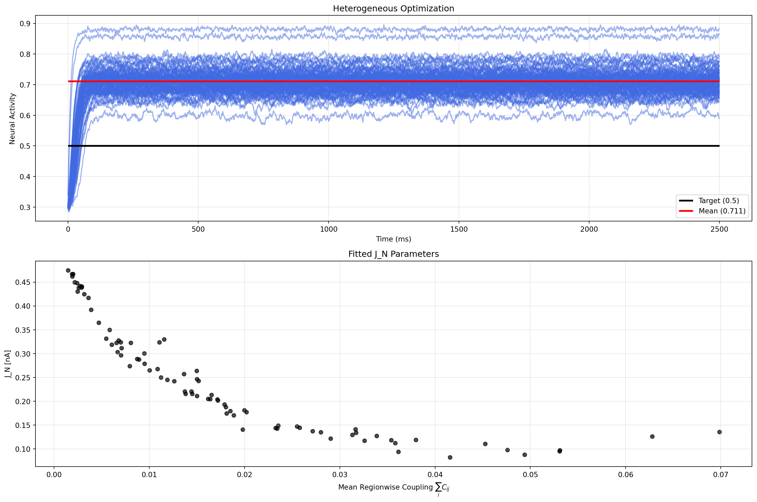
Now most regions are close to the target level after passing the initial transient. Setting the initial conditions to the target activity could be a solution to this problem.
::: {.panel-tabset}
## TVB-Optim
```{python}
#| echo: true
# Simulate with heterogeneous parameters
ts_optimized_het = model(optimized_state_het).data[:,0,:]
```
```{python}
#| echo: true
#| code-fold: true
#| code-summary: "Visualization"
plt.figure(figsize=(15, 10))

# Plot 1: Time series for all regions
plt.subplot(2, 1, 1)
plt.plot(ts_optimized_het, alpha = 0.5, color = "royalblue")
plt.hlines(0.5, 0, 2500, color = "black", linewidth = 2.5, label="Target (0.5)")
plt.hlines(observation(optimized_state_het), 0, 2500, color = "red", linewidth = 2.5,
           label=f"Mean ({observation(optimized_state_het):.3f})")
plt.xlabel("Time (ms)")
plt.ylabel("Neural Activity")
plt.title("Heterogeneous Optimization")
plt.legend()
plt.grid(True, alpha=0.3)

# Plot 2: J_N parameters vs mean regionwise coupling
mean_coupling = jnp.mean(weights, axis=1)
plt.subplot(2, 1, 2)
plt.scatter(mean_coupling, optimized_state_het.dynamics.J_N.value.flatten(), alpha=0.7, color="k", s=30)
plt.xlabel(r"Mean Regionwise Coupling $\sum_i C_{ij}$")
plt.ylabel("J_N [nA]")
plt.title("Fitted J_N Parameters")
plt.grid(True, alpha=0.3)

plt.tight_layout()
```
## TVB-O
```{python}
#| eval: false
#| echo: true
# Simulate with heterogeneous parameters
ts_optimized_het_tvbo = model_tvbo(optimized_state_het_tvbo)[0].data[:,0,:,0]
```
```{python}
#| eval: false
#| echo: true
#| code-fold: true
#| code-summary: "Visualization"
plt.figure(figsize=(15, 10))

# Plot 1: Time series for all regions
plt.subplot(2, 1, 1)
plt.plot(ts_optimized_het_tvbo, alpha = 0.5, color = "royalblue")
plt.hlines(0.5, 0, 2500, color = "black", linewidth = 2.5, label="Target (0.5)")
plt.hlines(observation_tvbo(optimized_state_het_tvbo), 0, 2500, color = "red", linewidth = 2.5,
           label=f"Mean ({observation_tvbo(optimized_state_het_tvbo):.3f})")
plt.xlabel("Time (ms)")
plt.ylabel("Neural Activity")
plt.title("Heterogeneous Optimization")
plt.legend()
plt.grid(True, alpha=0.3)

# Plot 2: J_N parameters vs mean regionwise coupling
mean_coupling = jnp.mean(experiment.connectivity.weights, axis=1)
plt.subplot(2, 1, 2)
plt.scatter(mean_coupling, optimized_state_het_tvbo.parameters.model.J_N.value.flatten(), alpha=0.7, color="k", s=30)
plt.xlabel(r"Mean Regionwise Coupling $\sum_i C_{ij}$")
plt.ylabel("J_N [nA]")
plt.title("Fitted J_N Parameters")
plt.grid(True, alpha=0.3)

plt.tight_layout()
```
:::
Why is this problem interesting? The Reduced Wong Wang model has two fixed point branches - low activity (~0.1) and high activity (~0.9). Each region tends to approach one of them, but for the desired target level, we need to find a balance between the two. This concept is also known as feedback inhibition control (FIC).
## Key Concepts Demonstrated
This tutorial showcased several important TVB-Optim concepts:
1. **Parameter Types**: The `Parameter` class wraps JAX arrays with additional functionality and constraints.
2. **State Management**: The state object is a JAX PyTree containing all simulation parameters and initial conditions
3. **Spaces**: `Space` enables systematic parameter exploration by flexibly placing `Axis` objects
4. **Execution Strategies**: `ParallelExecution` leverages JAX's pmap for efficient computation across parameter sets
5. **Optimization**: `OptaxOptimizer` provides gradient-based optimization with automatic differentiation
6. **Caching**: The `@cache` decorator saves expensive computations for reuse
7. **Heterogeneous Parameters**: Region-specific parameters enable fine-grained control over brain dynamics
These tools enable efficient exploration and optimization of complex brain network models at scale.