---
title: "Stimulation with Bayesian Inference"
subtitle: "Recovering Stimulus and Excitability from a Degenerate Forward Model"
format:
html:
code-fold: false
toc: true
echo: false
fig-width: 8
out-width: "100%"
jupyter: python3
execute:
cache: true
---
Try this notebook interactively:
[Download .ipynb](https://github.com/virtual-twin/tvboptim/blob/main/docs/workflows/Stimulation_with_Bayesian_Inference.ipynb){.btn .btn-primary download="Stimulation_with_Bayesian_Inference.ipynb"}
[Download .qmd](https://github.com/virtual-twin/tvboptim/blob/main/docs/workflows/Stimulation_with_Bayesian_Inference.qmd){.btn .btn-secondary download="Stimulation_with_Bayesian_Inference.qmd"}
[Open in Colab](https://colab.research.google.com/github/virtual-twin/tvboptim/blob/main/docs/workflows/Stimulation_with_Bayesian_Inference.ipynb){.btn .btn-warning target="_blank"}
## Introduction
A pulse stimulus is delivered to a `Generic2dOscillator` and we record a noisy time series. From that one recording, we want to recover two things: how strong the stimulus was, and how excitable the underlying system is. The problem is that these two parameters trade off. A weaker stimulus into a more excitable system produces almost the same trajectory as a stronger stimulus into a less excitable one.
Gradient descent picks an arbitrary point on this ridge of equally good fits and reports it as *the* answer. Bayesian inference reports the whole ridge, and prior knowledge about either parameter (a device log, a PET scan) shifts the posterior onto a specific segment of the ridge, with the prior's strength controlling how tight that segment is.
We run the example at a single node so the documentation renders in CI; the same construction applies node-by-node to a network.
::: {.callout-warning}
## What this notebook does not claim
- **Single-region by construction.** The forward model, prior, and posterior all live at one node. The extension to networks is mechanical (per-node parameters as `DataAxis`), but rendering a multi-region MCMC fit would dominate CI time.
- **The likelihood width is set deliberately wider than the data noise** (`LIKELIHOOD_SIGMA = 0.2` vs `OBS_NOISE_SIGMA = 0.1`). This is a didactic choice that keeps the likelihood flat along the ridge so the prior choice is visibly responsible for the difference between scenarios. With matched σ the posterior collapses harder onto the truth and the steering effect is harder to see. The next section unpacks this.
- **Priors here stand in for evidence sources.** We do not pull from a real PET map. Replacing `dist.Normal(PRIOR_AMP_MEAN, amp_std)` with `dist.Normal(mu_from_PET, sigma_from_PET)` is a one-line change, but this notebook does not work through an empirical example.
- **High-dim inference is mostly a hardware question.** Reverse-mode AD keeps the gradient cost almost flat in parameter count, so HMC on a thousand parameters runs given a GPU and a long-running workload. The real limit is posterior geometry (multimodality, conditioning), not raw dimension. The final section discusses what scales well and when to swap method.
:::
```{python}
#| output: false
#| echo: false
# Install dependencies if running in Google Colab
try:
import google.colab
print("Running in Google Colab - installing dependencies...")
!pip install -q tvboptim numpyro
print("✓ Dependencies installed!")
except ImportError:
pass # Not in Colab, assume dependencies are available
```
The notebook proceeds in four steps:
1. Generate a noisy observation from a known ground truth.
2. Scan the MSE landscape and show that many parameter pairs explain the data.
3. Sample three posteriors with different priors on the same observation.
4. Compare those posteriors against multi-start gradient descent on the same priors.
::: {.callout-tip}
## What you'll learn
- **Concepts:** what parameter degeneracy looks like, why a point estimate hides it, and how a prior turns "any answer on the ridge" into "the answer consistent with what you already know".
- **TVB-Optim idioms:** wiring `tvboptim` forward simulation into a `numpyro` model, using `GridAxis` for landscape scans, `DataAxis` to batch posterior-predictive draws.
- **Workflow:** what changes when you swap an optimizer for a sampler, and how to read the result.
:::
```{python}
#| output: false
#| code-fold: true
#| code-summary: "Environment Setup and Imports"
#| echo: true
# Set up environment — XLA_FLAGS must be set BEFORE importing jax. Here we expose
# 25 virtual devices so ParallelExecution can spread landscape scans, posterior
# predictive draws, and multi-start optimisations across many devices at once.
import os

N_DEVICES = 25
os.environ["XLA_FLAGS"] = f"--xla_force_host_platform_device_count={N_DEVICES}"

import numpy as np
import jax
import jax.numpy as jnp
import matplotlib.pyplot as plt
import numpyro
import numpyro.distributions as dist
import optax
from numpyro.infer import MCMC, NUTS
from numpyro.infer.util import log_density
from scipy.stats import gaussian_kde, iqr

from tvboptim.execution import ParallelExecution
from tvboptim.experimental.network_dynamics import Network, prepare, solve as nd_solve
from tvboptim.experimental.network_dynamics.dynamics.tvb import Generic2dOscillator
from tvboptim.experimental.network_dynamics.coupling import LinearCoupling
from tvboptim.experimental.network_dynamics.graph import DenseGraph
from tvboptim.experimental.network_dynamics.external_input import PulseInput
from tvboptim.experimental.network_dynamics.solvers import Heun
from tvboptim.types import DataAxis, GridAxis, Space, Parameter, collect_parameters
from tvboptim.optim import OptaxOptimizer
from tvboptim.utils import set_cache_path, cache

# Cache directory for expensive MCMC and optimisation runs
set_cache_path("./bayes_stim")
```
## Shared Settings and Priors
The three scenarios use identical prior **means** and differ only in their **standard deviations**. A tight prior on one parameter is how we tell the model that we already have evidence about it:
- **A**: no hypothesis. Wide priors on both parameters.
- **B** (H1, *higher excitability*): tight prior on amplitude. The stimulator log is trusted, so the data has to be explained via excitability.
- **C** (H2, *stronger stimulus*): tight prior on excitability. PET or gene-expression evidence pins excitability down, so the data has to be explained via amplitude.
```{python}
#| echo: true
#| output: false
T1 = 150.0
DT = 0.2
ONSET = 10.0
DURATION = 1.0

TRUE_AMPLITUDE = 0.4
TRUE_EXCITABILITY = 0.1
OBS_NOISE_SIGMA = 0.1    # data generation noise
LIKELIHOOD_SIGMA = 0.2   # fixed in likelihood — intentionally flat along ridge so priors steer

PRIOR_AMP_MEAN = 0.2
PRIOR_EXC_MEAN = 0.0

# Scenario priors — all share the same means; each hypothesis constrains one
# parameter with a tight σ:
#   A: no hypothesis.            Wide priors on both.
#   B: H1, higher excitability.  Tight amp prior → excitability has to explain.
#   C: H2, stronger stimulus.    Tight exc prior → amplitude has to explain.
PRIOR_AMP_STD = {"A": 0.20, "B": 0.10, "C": 0.20}
PRIOR_EXC_STD = {"A": 0.10, "B": 0.10, "C": 0.05}

SCENARIO_LABELS = {
    "A": "No hypothesis\n(wide priors on both)",
    "B": f"H1: Higher excitability\namp ~ N({PRIOR_AMP_MEAN}, {PRIOR_AMP_STD['B']})",
    "C": f"H2: Stronger stimulus\nexc ~ N({PRIOR_EXC_MEAN}, {PRIOR_EXC_STD['C']})",
}

DYNAMICS_PARAMS = dict(a=-1.5, b=-15.0, c=0.0, d=0.015, e=3.0, f=1.0, tau=4.0)
weights = jnp.zeros((1, 1))

SCENARIO_KEYS = ["A", "B", "C"]
COLORS = ["tab:blue", "tab:green", "tab:orange"]
```
## Stimulation in TVB-Optim: quick recap
The stimulus in this notebook is a rectangular pulse delivered to a single-node `Generic2dOscillator`. In TVB-Optim, stimuli live in the `external_input` slot of a `Network` and are routed by name. The dynamics class declares which names it accepts via its `EXTERNAL_INPUTS` attribute; for `Generic2dOscillator` the name is `'stimulus'`, and the value gets added into the equation for the fast variable `V`.
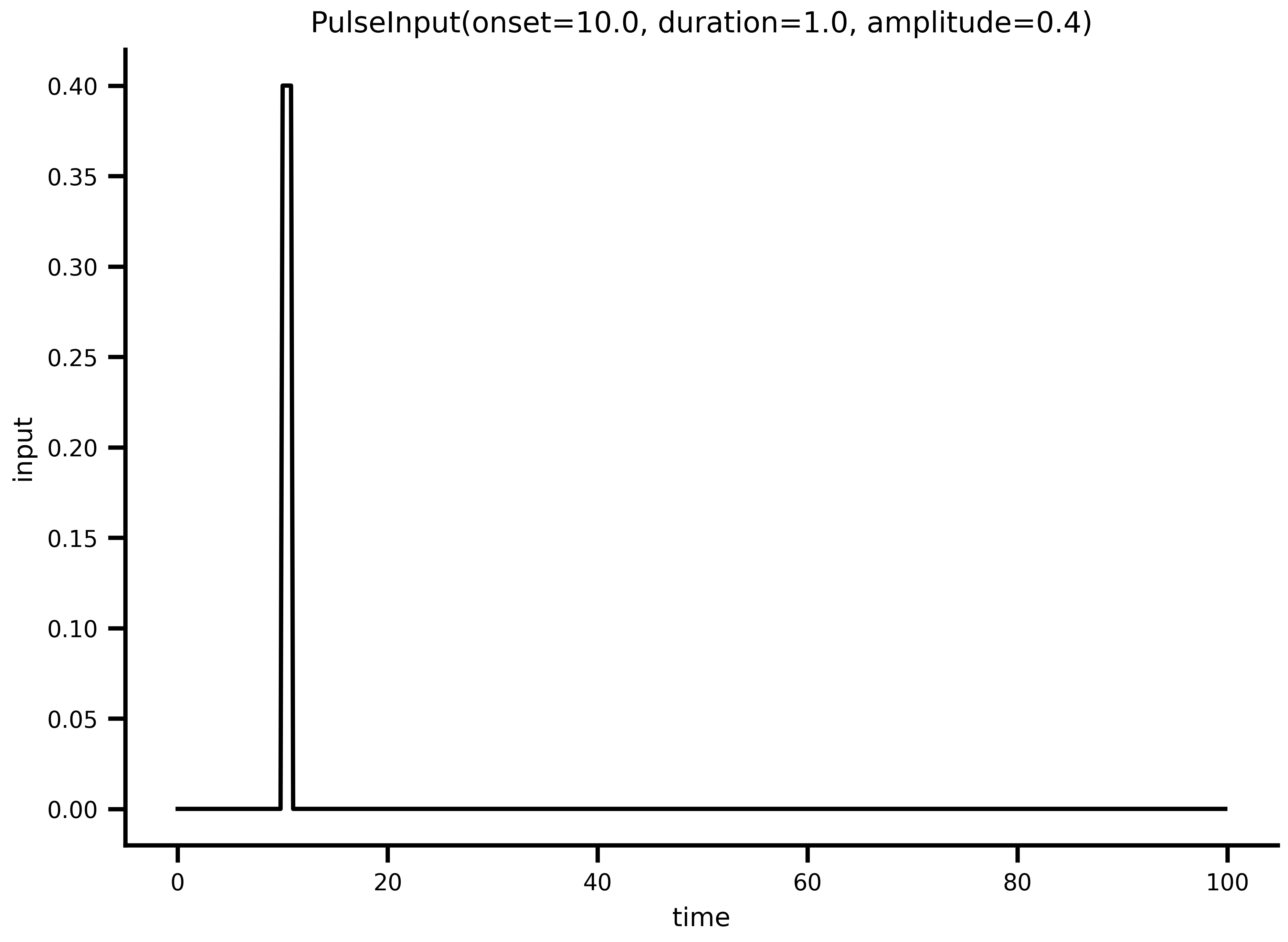
The pulse itself is a `PulseInput` parametrized by three numbers:
- `onset` — when the pulse starts (ms).
- `duration` — how long it stays on.
- `amplitude` — the constant value driving `V` during the on-window.
`PulseInput` is a *parametric* input: a function of time that the solver evaluates at each step. The alternative is `DataInput`, which interpolates between recorded samples; use it when you have an experimental stimulator trace rather than an idealized waveform. Any parameter of an external input can be wrapped in `Parameter(...)` to mark it as optimizable, which is exactly what we do later when comparing Bayesian inference against gradient descent.
In code, the wiring lives inside `build_network` (in the collapsed helpers block below):
```python
Network(
    dynamics=Generic2dOscillator(..., I=excitability, ...),
    coupling={"instant": LinearCoupling(...)},
    graph=DenseGraph(weights),
    external_input={"stimulus": PulseInput(
        onset=ONSET, duration=DURATION, amplitude=amplitude,
    )},
)
```
The name `"stimulus"` on the left of the dict has to match the name in `EXTERNAL_INPUTS`. The two free parameters of this notebook are `amplitude` (a property of the input) and `I` (a property of the dynamics, the excitability). They sit in different parts of the config, but the Bayesian model treats them symmetrically.
External inputs carry a `.plot()` method, which is the quickest way to confirm the pulse looks like what you wrote down:
```{python}
#| label: fig-stimulus
#| fig-cap: "**The pulse stimulus at the true parameters.** A 1 ms rectangular pulse of amplitude `TRUE_AMPLITUDE = 0.4` starting at `ONSET = 10 ms`. This is the time course added to the `V` equation of the `Generic2dOscillator` during the on-window."
#| echo: true
PulseInput(onset=ONSET, duration=DURATION, amplitude=TRUE_AMPLITUDE).plot(t0=0, t1=100)
```
## On the likelihood width
The data-generating noise is `OBS_NOISE_SIGMA = 0.1` but the likelihood is scored with `LIKELIHOOD_SIGMA = 0.2`. Why the mismatch?
A matched σ produces a posterior already tight enough around the truth that the prior choice barely moves it, hiding the demonstration. Inflating the likelihood σ keeps it flat along the degeneracy ridge, so the prior is what decides where the posterior concentrates. The trade-off is explicit: posteriors are *deliberately* wider than a maximum-likelihood analysis would produce. Try the run with `LIKELIHOOD_SIGMA = OBS_NOISE_SIGMA` and the ridge shortens but does not disappear, just over a narrower region.
## The Bayesian Model
This is what "transitioning from point estimates to full posteriors" looks like in code: the forward model is unchanged, the loss is replaced by a likelihood, and a sampler explores the joint of priors × likelihood. `make_model` returns a numpyro model that describes the joint distribution of parameters and data. Three things happen inside the inner `model` function:
1. **Priors.** `numpyro.sample("amplitude", dist.Normal(...))` draws an amplitude from the prior. It also tells numpyro: this is a latent variable named "amplitude", track its log-density. Same for excitability. The standard deviations `amp_std` and `exc_std` are scenario-specific and baked in from the closure.
2. **Forward simulation.** The sampled parameters are written into the simulation config and the forward model produces a predicted trajectory `v_pred`.
3. **Likelihood.** The final `numpyro.sample("obs", ..., obs=v_obs)` declares that the observation `v_obs` is a noisy version of `v_pred` with fixed noise scale `LIKELIHOOD_SIGMA`. The `obs=` keyword is what turns this from "sample obs" into "score obs against the model".
```{python}
#| echo: true
#| output: false
def make_model(scenario_key):
    """Return a numpyro model with scenario-specific prior widths baked in as closure constants."""
    amp_std = float(PRIOR_AMP_STD[scenario_key])
    exc_std = float(PRIOR_EXC_STD[scenario_key])

    def model(v_obs, solve_fn, config, obs_idx):
        # 1. Priors on the two latent parameters
        amplitude    = numpyro.sample("amplitude",    dist.Normal(PRIOR_AMP_MEAN, amp_std))
        excitability = numpyro.sample("excitability", dist.Normal(PRIOR_EXC_MEAN, exc_std))

        # 2. Forward simulation with the sampled parameters
        config.external.stimulus.amplitude = amplitude
        config.dynamics.I = excitability
        v_pred = solve_fn(config).ys[obs_idx, 0, 0]

        # 3. Likelihood: observation is v_pred + Gaussian noise
        numpyro.sample("obs", dist.Normal(v_pred, LIKELIHOOD_SIGMA), obs=v_obs)

    return model
```
NUTS then samples the joint posterior over `amplitude` and `excitability` by combining (1), (2), and (3). The sampler never sees the priors as Python objects: it only sees the resulting log-density. That is why `amp_std` and `exc_std` are converted to Python floats before being captured in the closure. Passing live `dist.Normal` objects in from the outside would break JIT tracing and silently drop the priors.
The model is decoupled from the sampler. The same `model` accepts three inference paths with no model change — pick by use case:
```python
# 1. NUTS — full posterior (this notebook's default; see run_mcmc in the helpers)
mcmc = MCMC(NUTS(model, dense_mass=True), num_warmup=500, num_samples=2000)
mcmc.run(rng, v_obs, sf, cfg, obs_idx)
posterior_samples = mcmc.get_samples()

# 2. SVI with an auto-guide — parametric posterior, much cheaper, less faithful in the tails
from numpyro.infer import SVI, Trace_ELBO, autoguide
guide = autoguide.AutoMultivariateNormal(model)
svi_result = SVI(model, guide, optax.adam(1e-2), Trace_ELBO()).run(
    rng, 2000, v_obs, sf, cfg, obs_idx,
)
svi_samples = guide.sample_posterior(rng, svi_result.params, sample_shape=(2000,))

# 3. MAP — same machinery, point estimate (the Bayesian relative of gradient descent)
map_run = SVI(model, autoguide.AutoDelta(model), optax.adam(1e-2), Trace_ELBO()).run(
    rng, 1000, v_obs, sf, cfg, obs_idx,
)
```
NUTS gives a faithful posterior but pays for it in gradient evaluations. SVI fits a parametric family — fast, but the family choice is a modelling decision and tail behaviour can be off. MAP recovers a point estimate within the same framework, and is conceptually what the multi-start optimisation later in this notebook approximates with a flat prior.
::: {.callout-note collapse="true"}
## Other helpers (network, loss, MCMC runner, plotting)
These are plumbing: the network factory, the MSE loss for the optimization comparison, the MCMC runner with NUTS settings, and a small landscape-drawing helper used by several figures.
```{python}
#| echo: true
#| output: false
def build_network(amplitude, excitability):
    """Deterministic forward model network."""
    return Network(
        dynamics=Generic2dOscillator(**DYNAMICS_PARAMS, I=excitability, VARIABLES_OF_INTEREST=("V",)),
        coupling={"instant": LinearCoupling(incoming_states="V", G=0.0)},
        graph=DenseGraph(weights),
        external_input={"stimulus": PulseInput(onset=ONSET, duration=DURATION, amplitude=amplitude)},
    )


def make_loss(solve_fn):
    """MSE loss against observed data, closed over solve_fn."""
    def loss(config):
        return jnp.mean((solve_fn(config).ys[obs_idx, 0, 0] - v_obs) ** 2)
    return loss


def run_mcmc(model_fn, seed, label, num_warmup=500, num_samples=2000, num_chains=1):
    print(f"\n{'='*60}\n{label}\n{'='*60}")
    net = build_network(TRUE_AMPLITUDE, TRUE_EXCITABILITY)
    sf, cfg = prepare(net, Heun(), t0=0.0, t1=T1, dt=DT)
    nuts = NUTS(
        model_fn,
        max_tree_depth=10,
        dense_mass=True,        # learns ridge correlation → explores along it
        target_accept_prob=0.8,
    )
    mcmc = MCMC(nuts, num_warmup=num_warmup, num_samples=num_samples, num_chains=num_chains)
    mcmc.run(jax.random.key(seed), v_obs, sf, cfg, obs_idx)
    mcmc.print_summary()
    return mcmc.get_samples(group_by_chain=False)


def _draw_landscape(ax, vmax=None):
    """Draw MSE heatmap + 10th-percentile contour + ground truth marker; return pcm."""
    pcm = ax.pcolormesh(amp_vals, excit_vals, mse_grid,
                        cmap="cividis_r", vmax=vmax or vmax_clip)
    ax.contour(amp_vals, excit_vals, mse_grid,
               levels=[float(jnp.percentile(mse_grid, 10))],
               colors="white", linewidths=1.0, linestyles="--")
    ax.scatter(TRUE_AMPLITUDE, TRUE_EXCITABILITY,
               color="white", marker="*", s=260, zorder=8,
               edgecolors="k", linewidths=1., label="ground truth")
    ax.set_xlabel("Stimulus amplitude")
    ax.set_ylabel("Excitability (I)")
    # Clamp axes to the scanned landscape extent so later scatter() calls
    # (posterior samples, optimisation endpoints) don't trigger autoscale.
    ax.set_xlim(float(amp_vals[0]),   float(amp_vals[-1]))
    ax.set_ylim(float(excit_vals[0]), float(excit_vals[-1]))
    return pcm
```
:::
## Generating the Observation
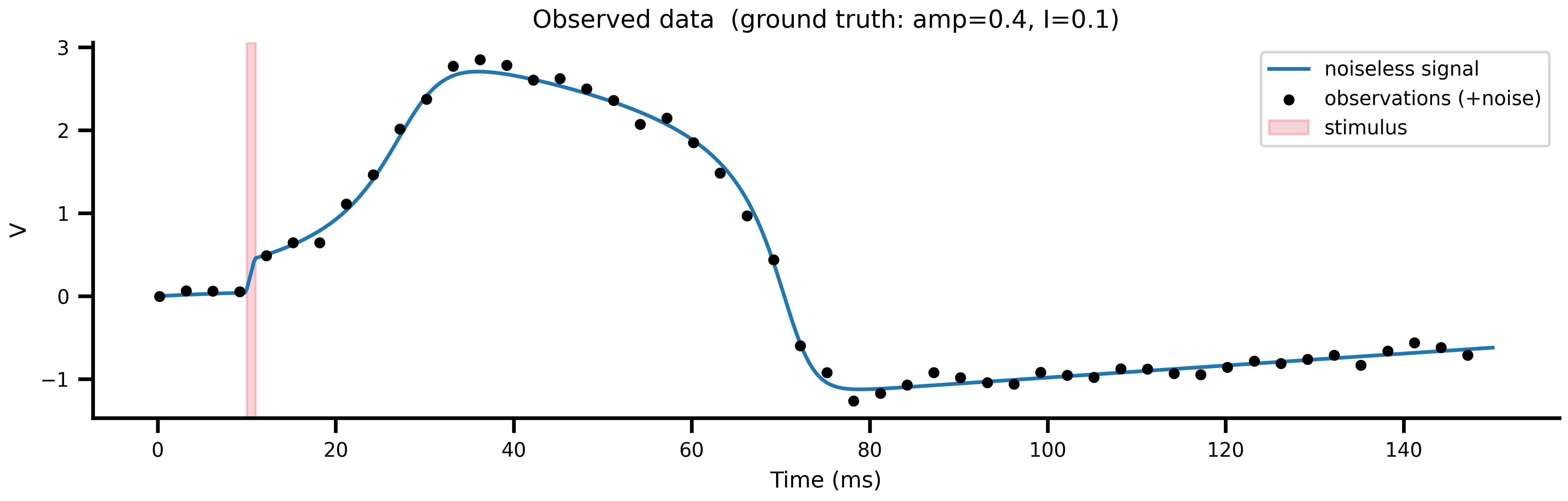
Simulate the forward model at the true parameters, subsample every 15 steps, add Gaussian noise. The noiseless trajectory is kept around as the reference for MSE in the landscape scan that follows.
```{python}
#| echo: true
#| output: false
# Noiseless signal as base ensures MLE at true params. Ridge points produce near-identical
# noiseless signals, so the likelihood is flat along the ridge and priors steer freely.
network_true = build_network(TRUE_AMPLITUDE, TRUE_EXCITABILITY)
solve_true, config_true = prepare(network_true, Heun(), t0=0.0, t1=T1, dt=DT)
v_noiseless = solve_true(config_true).ys[:, 0, 0]
ts = solve_true(config_true).ts

obs_idx = jnp.arange(0, len(ts), 15)
ts_obs = ts[obs_idx]
v_obs = v_noiseless[obs_idx] + OBS_NOISE_SIGMA * jax.random.normal(
    jax.random.key(42), (len(obs_idx),)
)
```
```{python}
#| label: fig-observation
#| fig-cap: "**Observed data and underlying signal.** Blue: noiseless ground-truth trajectory at `amp=0.4, I=0.1`. Black points: subsampled observations with additive Gaussian noise. Red band: the stimulus pulse window."
#| code-fold: true
#| code-summary: "Show plotting code"
fig, ax = plt.subplots(figsize=(9, 3))
ax.plot(ts, v_noiseless, color="tab:blue", lw=1.5, label="noiseless signal")
ax.scatter(ts_obs, v_obs, s=12, color="k", zorder=3, label="observations (+noise)")
ax.axvspan(ONSET, ONSET + DURATION, alpha=0.2, color="tab:red", label="stimulus")
ax.set_xlabel("Time (ms)")
ax.set_ylabel("V")
ax.set_title(f"Observed data (ground truth: amp={TRUE_AMPLITUDE}, I={TRUE_EXCITABILITY})")
ax.legend()
fig.tight_layout()
```
## Mapping the Loss Landscape
Before any inference, scan the 2D parameter space and compute MSE between the deterministic simulation and the noiseless target at each grid point. The result is the *degeneracy landscape*: the set of `(amplitude, excitability)` pairs the data cannot distinguish.
```{python}
#| echo: true
#| output: false
N_AMP = N_DEVICES
N_EXCIT = N_DEVICES

net_scan = build_network(TRUE_AMPLITUDE, TRUE_EXCITABILITY)
sf_scan, cfg_scan = prepare(net_scan, Heun(), t0=0.0, t1=T1, dt=DT)

cfg_scan.external.stimulus.amplitude = GridAxis(0.0, 1.0, N_AMP)
cfg_scan.dynamics.I = GridAxis(-0.1, 0.5, N_EXCIT)
space = Space(cfg_scan, mode="product")

par = ParallelExecution(
    model=lambda cfg: sf_scan(cfg).ys[:, 0, 0],
    space=space, n_pmap=N_DEVICES, n_vmap=N_DEVICES,
)
scan_results = par.run()
print("Landscape scan complete.")

df_scan = scan_results.to_dataframe()
amp_vals   = jnp.array(sorted(df_scan["external.stimulus.amplitude"].unique()))
excit_vals = jnp.array(sorted(df_scan["dynamics.I"].unique()))

mse_grid = jnp.zeros((len(excit_vals), len(amp_vals)))
for row_idx, row in df_scan.iterrows():
    mse   = float(jnp.mean((scan_results[row_idx] - v_noiseless) ** 2))
    i_amp = int(jnp.argmin(jnp.abs(amp_vals   - row["external.stimulus.amplitude"])))
    i_ex  = int(jnp.argmin(jnp.abs(excit_vals - row["dynamics.I"])))
    mse_grid = mse_grid.at[i_ex, i_amp].set(mse)

vmax_clip = float(jnp.percentile(mse_grid, 75))
```
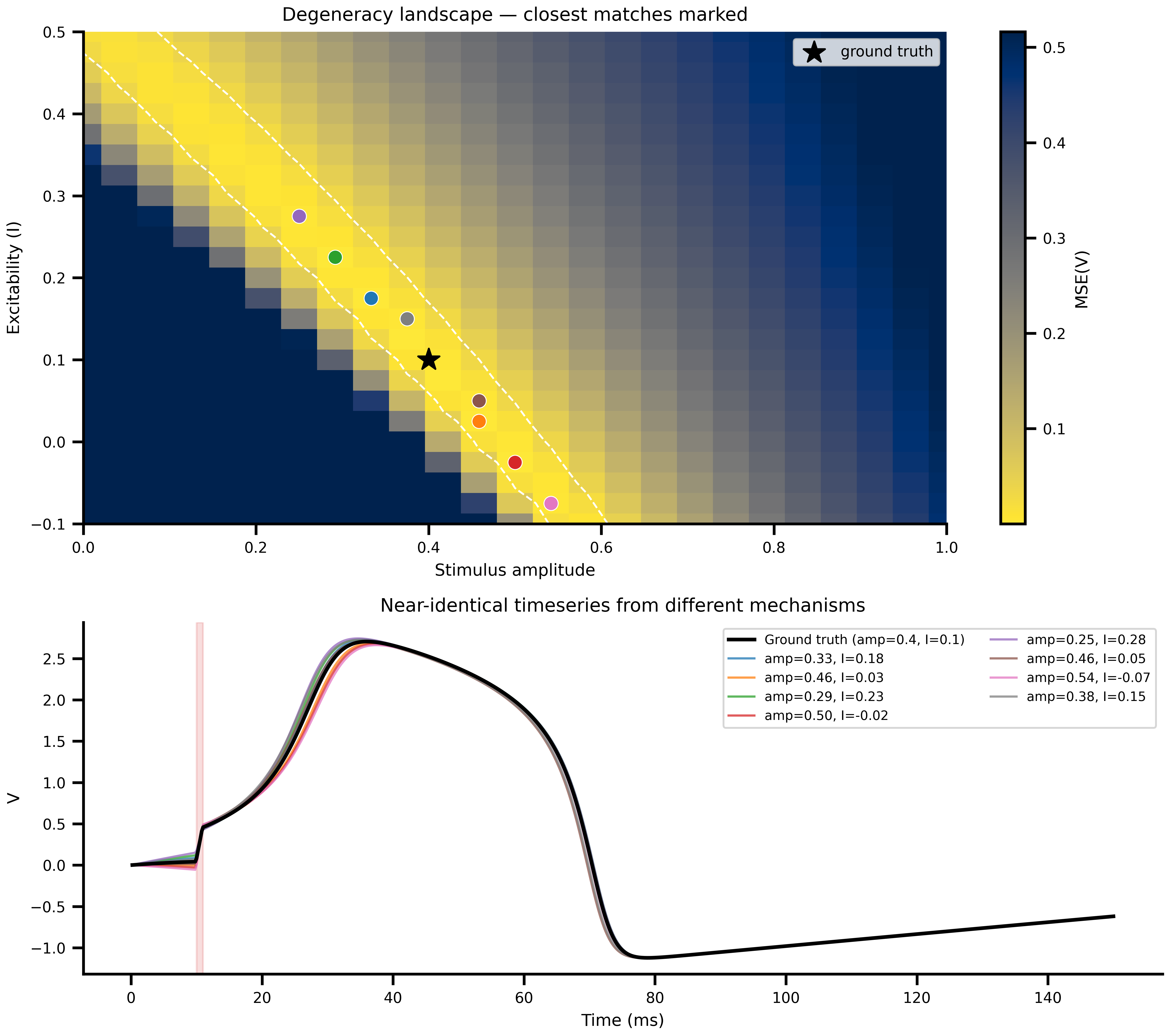
Pick the eight lowest-MSE grid points (excluding a small neighborhood of the ground truth) and overlay their simulated trajectories. They are visually nearly identical despite coming from qualitatively different mechanistic explanations.
```{python}
#| label: fig-degeneracy
#| fig-cap: "**The degeneracy ridge.** Top: MSE landscape with the eight lowest-loss off-truth grid points marked. Bottom: their simulated trajectories overlaid on the ground truth. They are visually almost identical despite different `(amp, I)` combinations. This is the ambiguity any inference method has to deal with."
#| code-fold: true
#| code-summary: "Show plotting code"
N_MATCHES = 8
cmap_matches = plt.get_cmap("tab10")
sorted_idx = jnp.argsort(mse_grid.flatten())
matches = []
for flat_idx in sorted_idx:
if len(matches) >= N_MATCHES:
break
i_ex = int(flat_idx) // N_AMP
i_amp = int(flat_idx) % N_AMP
amp = float(amp_vals[i_amp])
excit = float(excit_vals[i_ex])
if abs(amp - TRUE_AMPLITUDE) < 0.05 and abs(excit - TRUE_EXCITABILITY) < 0.05:
continue
net_m = build_network(amp, excit)
sf_m, cfg_m = prepare(net_m, Heun(), t0=0.0, t1=T1, dt=DT)
matches.append((amp, excit, sf_m(cfg_m).ys[:, 0, 0]))
fig, (ax_map, ax_ts) = plt.subplots(2, 1, figsize=(9, 8),
gridspec_kw={"height_ratios": [1.4, 1]})
pcm = _draw_landscape(ax_map)
fig.colorbar(pcm, ax=ax_map, label="MSE(V)")
for idx, (amp, excit, _) in enumerate(matches):
ax_map.scatter(amp, excit, color=cmap_matches(idx), s=60, zorder=5,
edgecolors="white", linewidths=0.5)
ax_map.set_title("Degeneracy landscape — closest matches marked")
ax_map.legend(fontsize=8)
ax_ts.plot(ts, v_noiseless, color="black", lw=2,
label=f"Ground truth (amp={TRUE_AMPLITUDE}, I={TRUE_EXCITABILITY})", zorder=10)
ax_ts.axvspan(ONSET, ONSET + DURATION, alpha=0.15, color="tab:red")
for idx, (amp, excit, v_m) in enumerate(matches):
ax_ts.plot(ts, v_m, color=cmap_matches(idx), alpha=0.75, lw=1.2,
label=f"amp={amp:.2f}, I={excit:.2f}")
ax_ts.set_ylabel("V")
ax_ts.set_xlabel("Time (ms)")
ax_ts.set_title("Near-identical timeseries from different mechanisms")
ax_ts.legend(fontsize=7, ncol=2)
fig.tight_layout()
```
## Identifiability from autodiff: the same ridge, in one gradient call
The 25 × 25 scan above maps the ridge by brute force — 625 forward simulations to expose the geometry the optimiser runs into on every step. The gradients that drive optimisation give that geometry analytically. Take the Jacobian of the predicted trajectory w.r.t. `(amplitude, I)`, form `J^T J / σ²` (the Gauss-Newton Fisher information), eigendecompose. The smallest-eigenvalue eigenvector is the local ridge tangent; the eigenvalue ratio quantifies how much flatter the ridge is than the cross-ridge direction. Cost: one forward + one reverse-mode pass, independent of parameter count.
One small but important detail: the input to `fisher_information` is the model's **prediction vector**, not the scalar loss. The Jacobian `J = ∂(predictions) / ∂θ` lives one level *above* the reduction to MSE — once the loss has summed over the observation index, that sensitivity information is gone. So `predict` below returns the predicted observation directly. The same pattern applies to any other observable: a BOLD time series, a flattened functional-connectivity matrix, summary statistics — anything the model emits before it gets compared to data.
```{python}
#| echo: true
from tvboptim.analysis import eigendecompose_curvature, fisher_information

net_id = build_network(TRUE_AMPLITUDE, TRUE_EXCITABILITY)
sf_id, cfg_id = prepare(net_id, Heun(), t0=0.0, t1=T1, dt=DT)
cfg_id.external.stimulus.amplitude = Parameter(TRUE_AMPLITUDE)
cfg_id.dynamics.I = Parameter(TRUE_EXCITABILITY)

# The predicted observation as a vector — one entry per observation time.
# `fisher_information` takes ∂predict/∂θ for the two Parameter leaves;
# σ = OBS_NOISE_SIGMA puts the resulting FIM in Cramér-Rao units.
def predict(c):
    return sf_id(c).ys[obs_idx, 0, 0]

FIM, theta0, labels = fisher_information(predict, cfg_id, sigma=OBS_NOISE_SIGMA)
result = eigendecompose_curvature(FIM, labels, theta0, kind="fisher")
print(result.summary())
```
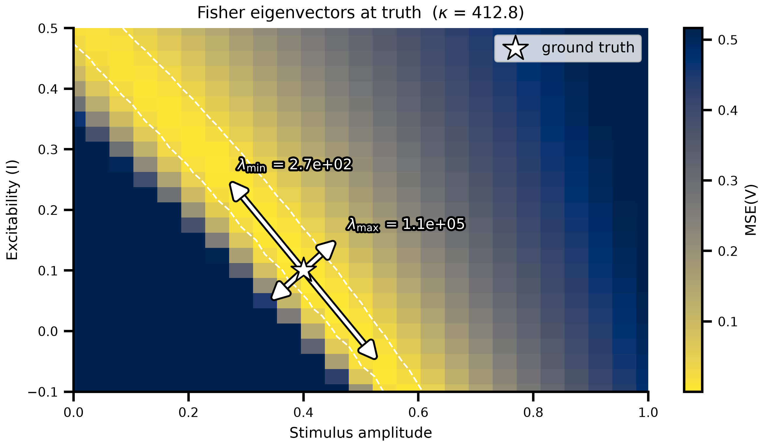
The sloppy direction comes out with opposite signs on the two parameters — `dynamics.I` at −0.75 and `external.stimulus.amplitude` at +0.66 — exactly the "more excitable + weaker stimulus" trade-off the grid scan revealed. The condition number κ ≈ 413 quantifies it: the cross-ridge direction (eigenvalue ≈ 1.1 × 10⁵) is constrained by the data more than two orders of magnitude tighter than the along-ridge one (eigenvalue ≈ 2.7 × 10²). Numerical rank is 2 / 2, so both parameters are *technically* identifiable at this noise scale; the diagnostic flags the disparity in confidence between the two directions, not absolute non-identifiability. That distinction matters for the rebuttal: a practical identifiability problem can hide inside a model that is structurally identifiable, and only the eigenvalue spread exposes it.
```{python}
#| label: fig-fisher-ridge
#| fig-cap: "**Fisher eigenstructure overlaid on the MSE landscape.** Long arrow: the smallest-eigenvalue (sloppy) eigenvector of `J^T J` at truth — it traces the equal-MSE ridge that the 25 × 25 scan exposes. Short arrow: the largest-eigenvalue (stiff) eigenvector, perpendicular to the ridge and orders of magnitude more tightly constrained by the data. Tip labels give the eigenvalues; their ratio is the condition number in the title."
#| code-fold: true
#| code-summary: "Show plotting code"
from matplotlib.patches import FancyArrowPatch
from matplotlib import patheffects as pe
i_amp = result.labels.index("external.stimulus.amplitude")
i_exc = result.labels.index("dynamics.I")
v_sloppy = np.asarray(result.eigenvectors[:, 0])
v_stiff = np.asarray(result.eigenvectors[:, -1])
lam_min = float(result.eigenvalues[0])
lam_max = float(result.eigenvalues[-1])
fig, ax = plt.subplots(figsize=(7, 4), dpi=200)
pcm = _draw_landscape(ax)
fig.colorbar(pcm, ax=ax, label="MSE(V)")
def _draw_eigenvector(v, L, label):
"""White-fill / black-outlined double-headed arrow along v, labelled at the upper tip."""
dx = L * float(v[i_amp])
dy = L * float(v[i_exc])
arrow = FancyArrowPatch(
(TRUE_AMPLITUDE - dx, TRUE_EXCITABILITY - dy),
(TRUE_AMPLITUDE + dx, TRUE_EXCITABILITY + dy),
arrowstyle="<|-|>", mutation_scale=20,
color="white", lw=2.2, zorder=7,
)
arrow.set_path_effects([
pe.Stroke(linewidth=4.5, foreground="black"),
pe.Normal(),
])
ax.add_patch(arrow)
# Label at whichever tip has higher excitability (keeps text off the lower axis).
tip_x = TRUE_AMPLITUDE + (dx if dy >= 0 else -dx)
tip_y = TRUE_EXCITABILITY + (dy if dy >= 0 else -dy)
ax.annotate(
label,
xy=(tip_x, tip_y),
xytext=(6, 6), textcoords="offset points",
fontsize=9, color="white", zorder=8,
path_effects=[pe.withStroke(linewidth=2.5, foreground="black")],
)
# Sloppy arrow longer; stiff shorter — the numerical eigenvalues at the tips
# carry the exact magnitudes (visual length is just a fixed cue).
_draw_eigenvector(v_sloppy, L=0.20, label=fr"$\lambda_{{\min}}$ = {lam_min:.1e}")
_draw_eigenvector(v_stiff, L=0.08, label=fr"$\lambda_{{\max}}$ = {lam_max:.1e}")
ax.legend(fontsize=9, loc="upper right")
ax.set_title(
f"Fisher eigenvectors at truth "
fr"($\kappa$ = {result.condition_number():.1f})",
fontsize=10,
)
fig.tight_layout()
```
Two things matter for the rebuttal:
1. **The local diagnostic recovers the global ridge.** At a single point, autodiff produces the same trade-off direction the grid scan shows. That holds because the ridge is locally near-linear — but the test is empirical: the green line lies along the white dashed low-MSE contour the brute-force scan drew.
2. **It scales where the scan does not.** A 25 × 25 grid in two parameters is 625 simulations. The same diagnostic in `N` parameters is still one forward + one reverse pass; the dense `J^T J` is `O(N²)` to materialise, which is fine up to a few hundred parameters and can be replaced by a matrix-free Lanczos pass beyond that.
The eigenspectrum is local — it describes the basin around the supplied point only and will not see disconnected alternative optima. That is what MCMC gives you in the next sections. Identifiability analysis and posterior sampling answer different questions: *what shape is the basin* (cheap, local, AD-only) vs. *what does the data plus prior actually believe* (expensive, global, requires a likelihood and a sampler). Stacking them — local diagnostic first, then MCMC — is the cheapest path to a defensible uncertainty story.
## Sanity-Checking the Priors
Long MCMC runs hide silent bugs. Before launching one, evaluate the log joint density at two points under scenario C (tight excitability prior). A point with high `|I|` should score much worse than one with low `|I|` if the tight prior is actually active. If the two scores come out similar, the priors were dropped during tracing and the whole experiment is wrong.
```{python}
#| echo: true
_net_chk = build_network(TRUE_AMPLITUDE, TRUE_EXCITABILITY)
_sf_chk, _cfg_chk = prepare(_net_chk, Heun(), t0=0.0, t1=T1, dt=DT)
_args = (v_obs, _sf_chk, _cfg_chk, obs_idx)

# model_C has tight excitability prior → high-|I| points should score worse
_model_C = make_model("C")
lp_low,  _ = log_density(_model_C, _args, {}, {"amplitude": 0.5, "excitability": 0.0})
lp_high, _ = log_density(_model_C, _args, {}, {"amplitude": 0.1, "excitability": 0.3})
print(f"model_C  log p(amp=0.50, I=0.0):  {lp_low:.1f}")
print(f"model_C  log p(amp=0.10, I=0.3):  {lp_high:.1f}")
print(f"Difference: {lp_low - lp_high:.1f}  (should be >> 0 if tight exc prior is active)")
```
## Running MCMC Under Three Hypotheses
Sample three posteriors with NUTS. `dense_mass=True` matters here: the posterior is a thin diagonal ridge, and a learned full mass matrix lets the sampler step along the ridge instead of zig-zagging across it.
```{python}
#| echo: true
#| output: false
MCMC_KWARGS = dict(num_warmup=500, num_samples=4000, num_chains=1)

# @cache stores the function's return value on disk. On rerun the cached samples
# are loaded instead of resampling — set redo=True to force re-running the chain
# (e.g. after changing the priors or likelihood).
@cache("mcmc_samples", redo=False)
def run_all_mcmc():
    return [
        run_mcmc(make_model("A"), seed=0, label="A: No hypothesis (uninformative priors)", **MCMC_KWARGS),
        run_mcmc(make_model("B"), seed=1, label="H1: Higher excitability (e.g. PET, gene expression)", **MCMC_KWARGS),
        run_mcmc(make_model("C"), seed=2, label="H2: Stronger stimulus (e.g. device logs, protocol)", **MCMC_KWARGS),
    ]

all_samples = run_all_mcmc()
```
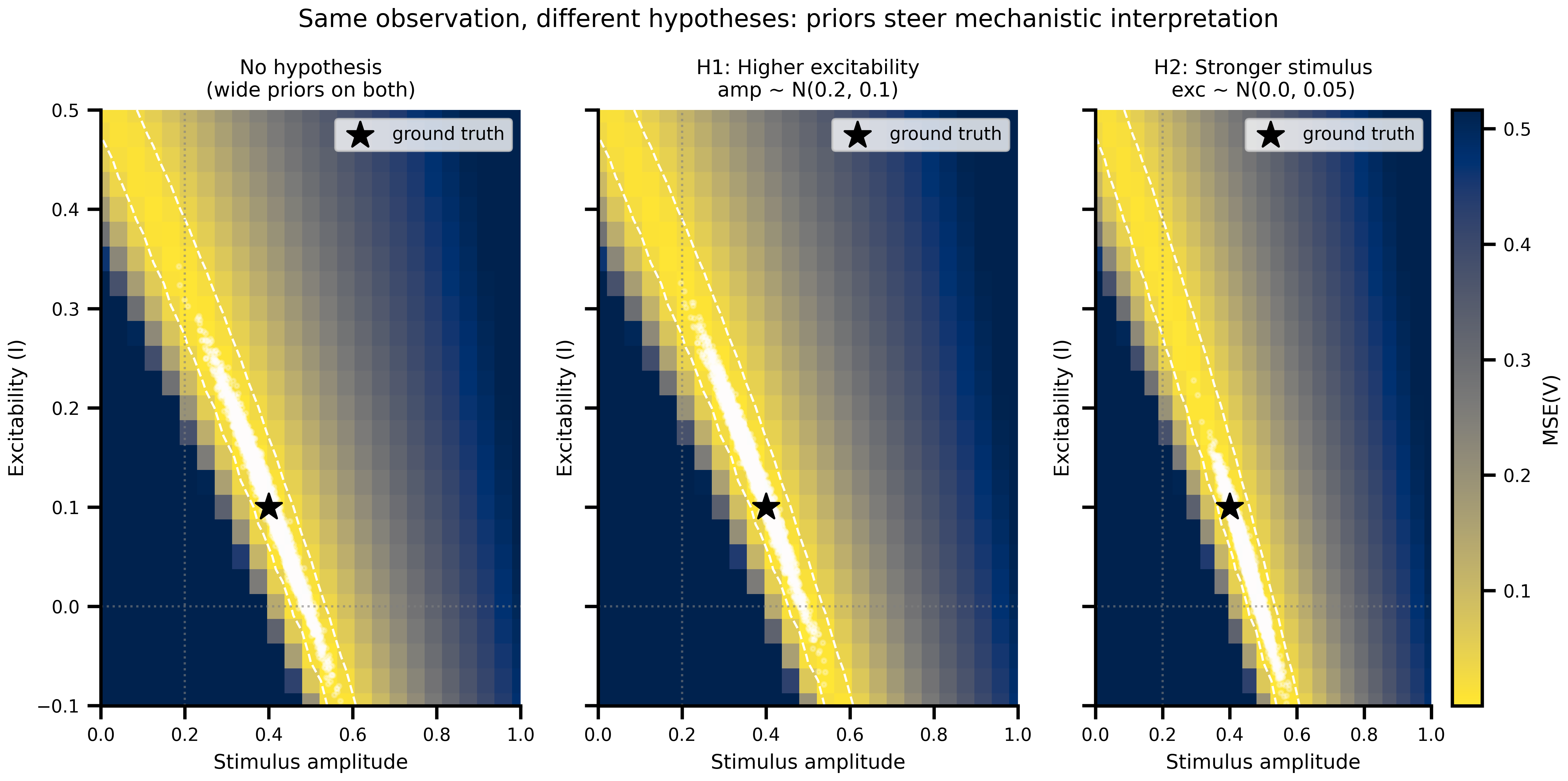
```{python}
#| label: fig-joint-posteriors
#| fig-cap: "**Joint posteriors overlaid on the degeneracy landscape.** Same observation, three hypotheses. Wide priors (A) let samples sprawl along the entire ridge; the tight-amplitude prior (B) confines them to a high-excitability segment; the tight-excitability prior (C) confines them to a high-amplitude segment. The data has not changed across panels, only the slice of the ridge the model is allowed to consider."
#| code-fold: true
#| code-summary: "Show plotting code"
fig, axes = plt.subplots(1, 3, figsize=(10, 5), sharey=True)
for ax, samples, key in zip(axes, all_samples, SCENARIO_KEYS):
pcm = _draw_landscape(ax)
ax.scatter(samples["amplitude"], samples["excitability"],
s=4, alpha=0.25, color="white", rasterized=True)
ax.axvline(PRIOR_AMP_MEAN, color="gray", ls=":", lw=1.0, alpha=0.6)
ax.axhline(PRIOR_EXC_MEAN, color="gray", ls=":", lw=1.0, alpha=0.6)
ax.set_title(SCENARIO_LABELS[key], fontsize=9)
ax.legend(fontsize=8)
axes[0].set_ylabel("Excitability (I)")
fig.colorbar(pcm, ax=axes[-1], label="MSE(V)")
fig.suptitle("Same observation, different hypotheses: priors steer mechanistic interpretation",
fontsize=11)
fig.tight_layout()
```
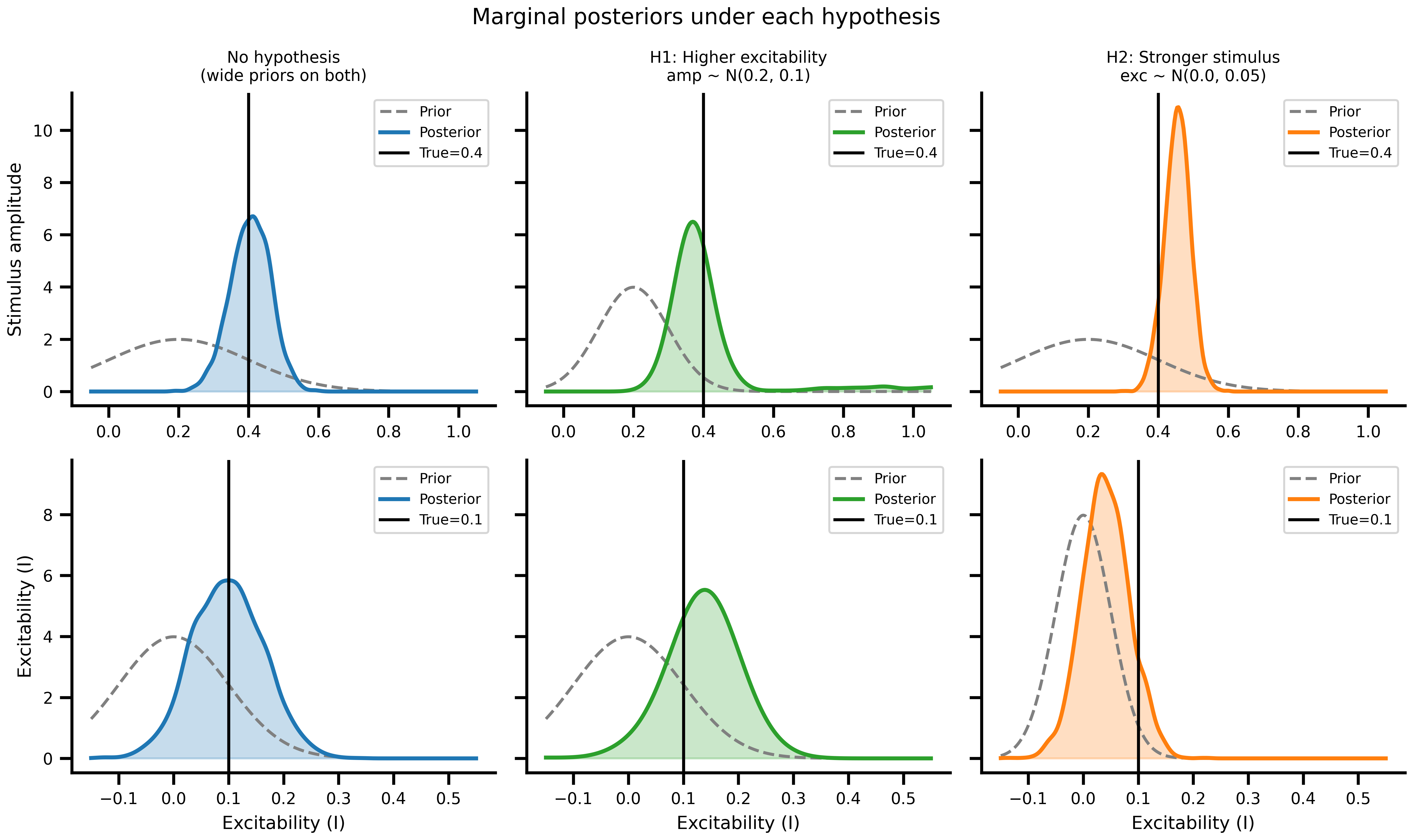
```{python}
#| label: fig-marginals
#| fig-cap: "**Marginal posteriors versus priors.** Dashed grey: prior density. Solid coloured: posterior KDE. Black: ground truth. Top row: amplitude; bottom row: excitability. A wide prior produces a data-driven posterior. A tight prior produces a posterior that tracks the prior, and the *other* parameter shifts to absorb the discrepancy."
#| code-fold: true
#| code-summary: "Show plotting code"
fig, axes = plt.subplots(2, 3, figsize=(10, 6), sharex="row", sharey="row")
param_meta = [
("amplitude", TRUE_AMPLITUDE, "Stimulus amplitude",
[dist.Normal(PRIOR_AMP_MEAN, PRIOR_AMP_STD[k]) for k in SCENARIO_KEYS],
amp_vals),
("excitability", TRUE_EXCITABILITY, "Excitability (I)",
[dist.Normal(PRIOR_EXC_MEAN, PRIOR_EXC_STD[k]) for k in SCENARIO_KEYS],
excit_vals),
]
for row, (param, true_val, xlabel, priors, grid) in enumerate(param_meta):
x = jnp.linspace(float(grid.min()) - 0.05, float(grid.max()) + 0.05, 300)
for col, (samples, key, prior, color) in enumerate(
zip(all_samples, SCENARIO_KEYS, priors, COLORS)
):
ax = axes[row, col]
kde = gaussian_kde(samples[param])
ax.plot(x, jnp.exp(prior.log_prob(x)), color="gray", ls="--", lw=1.5, label="Prior")
ax.plot(x, kde(x), color=color, lw=2, label="Posterior")
ax.fill_between(x, kde(x), alpha=0.25, color=color)
ax.axvline(true_val, color="k", lw=1.5, label=f"True={true_val}")
if row == 0:
ax.set_title(SCENARIO_LABELS[key], fontsize=8)
if col == 0:
ax.set_ylabel(xlabel, fontsize=9)
if row == 1:
ax.set_xlabel(xlabel, fontsize=9)
ax.legend(fontsize=7)
fig.suptitle("Marginal posteriors under each hypothesis", fontsize=11)
fig.tight_layout()
```
## Posterior Predictive
Push the posterior back through the forward model: draw `N_PP_DRAWS` parameter pairs per scenario, simulate each one, overlay the trajectories. The spread of the resulting ensemble is the model's uncertainty about future observations under that hypothesis, expressed in the same units as the data.
```{python}
#| echo: true
#| output: false
# Semi-transparent traces from posterior draws → uncertainty spread;
# posterior-mean prediction as solid line → point summary.
N_PP_DRAWS = 2 * N_DEVICES  # must be divisible into N_DEVICES × n_vmap

pp_traces = {}
pp_means  = {}

for key, samples in zip(SCENARIO_KEYS, all_samples):
    n_total  = len(samples["amplitude"])
    draw_idx = jnp.linspace(0, n_total - 1, N_PP_DRAWS).astype(int)

    net_pp = build_network(TRUE_AMPLITUDE, TRUE_EXCITABILITY)
    sf_pp, cfg_pp = prepare(net_pp, Heun(), t0=0.0, t1=T1, dt=DT)

    cfg_pp.external.stimulus.amplitude = DataAxis(samples["amplitude"][draw_idx])
    cfg_pp.dynamics.I                  = DataAxis(samples["excitability"][draw_idx])
    space_pp = Space(cfg_pp, mode="zip")

    par_pp = ParallelExecution(
        model=lambda cfg: sf_pp(cfg).ys[:, 0, 0],
        space=space_pp, n_pmap=N_DEVICES, n_vmap=N_PP_DRAWS // N_DEVICES,
    )
    results = par_pp.run()
    pp_traces[key] = jnp.array([results[i] for i in range(N_PP_DRAWS)])
    pp_means[key]  = (float(jnp.mean(samples["amplitude"])),
                      float(jnp.mean(samples["excitability"])))

print("Posterior predictive simulations complete.")
```
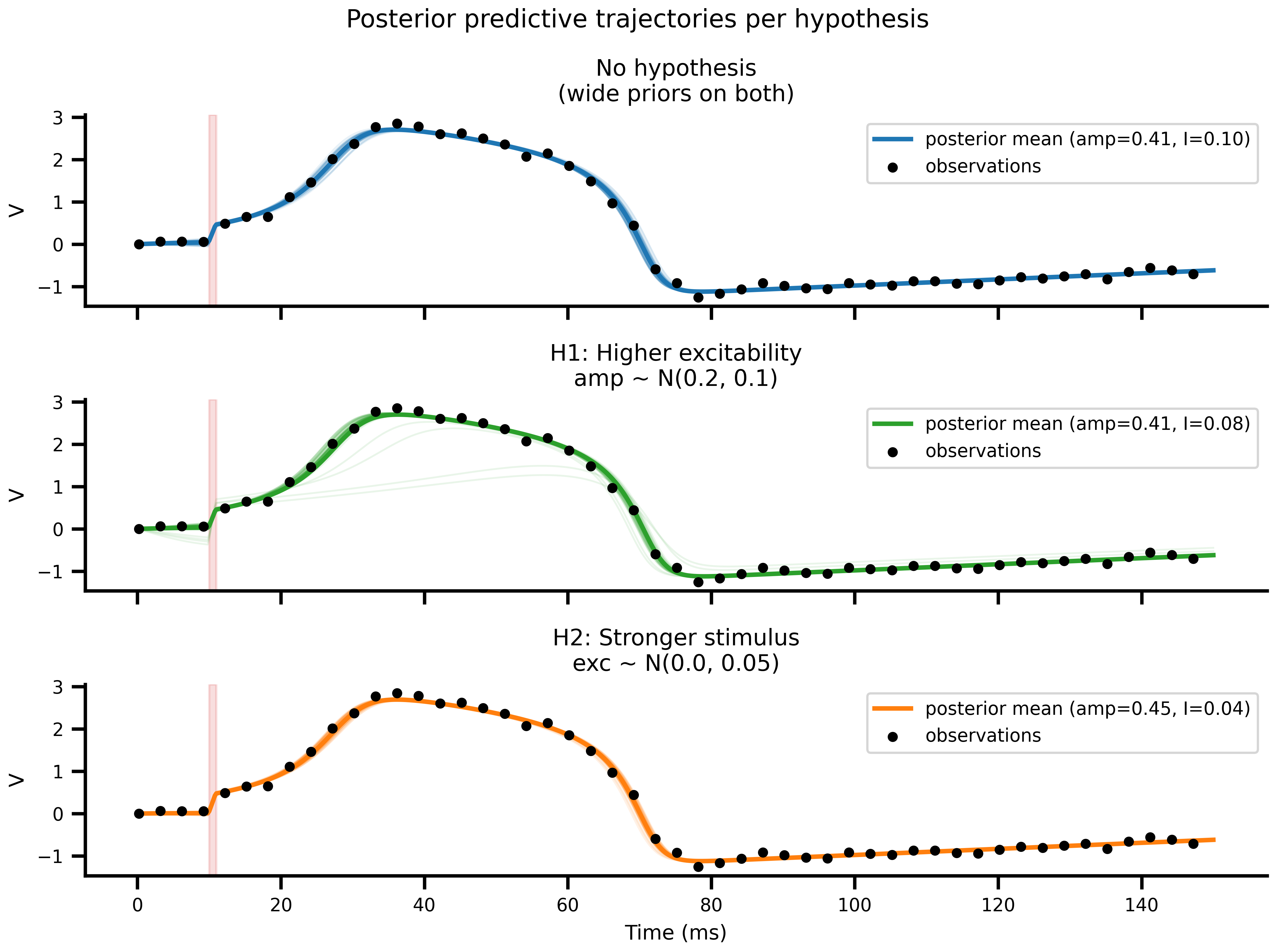
```{python}
#| label: fig-posterior-predictive
#| fig-cap: "**Posterior-predictive simulations.** Faint coloured lines: forward simulations from individual posterior draws. Solid coloured line: simulation at the posterior mean. Black dots: the original observations. All three scenarios fit the data equally well. They disagree only on *why*."
#| code-fold: true
#| code-summary: "Show plotting code"
fig, axes = plt.subplots(3, 1, figsize=(8, 6), sharex=True, sharey=True)
for ax, key, color in zip(axes, SCENARIO_KEYS, COLORS):
for i in range(N_PP_DRAWS):
ax.plot(ts, pp_traces[key][i], color=color, alpha=0.1, lw=0.8)
amp_mean, exc_mean = pp_means[key]
r_mean = nd_solve(build_network(amp_mean, exc_mean), Heun(), t0=0.0, t1=T1, dt=DT)
ax.plot(ts, r_mean.ys[:, 0, 0], color=color, lw=2.0,
label=f"posterior mean (amp={amp_mean:.2f}, I={exc_mean:.2f})")
ax.scatter(ts_obs, v_obs, s=12, color="k", zorder=5, label="observations")
ax.axvspan(ONSET, ONSET + DURATION, alpha=0.15, color="tab:red")
ax.set_ylabel("V")
ax.set_title(SCENARIO_LABELS[key], fontsize=10)
ax.legend(fontsize=8)
axes[-1].set_xlabel("Time (ms)")
fig.suptitle("Posterior predictive trajectories per hypothesis", fontsize=11)
fig.tight_layout()
```
## Comparison: Multi-Start Optimization
Skip Bayesian inference and run gradient descent instead. Sample starting points from each scenario's prior, run Adam for 1000 steps from each one. Every run collapses to a single point on the ridge. The optimizer cannot represent the residual uncertainty, and the starting distribution (the prior) decides which segment of the ridge each run lands in.
```{python}
#| echo: true
#| output: false
# Gradient descent from prior-sampled starts reveals:
# (a) each run converges to a single point on the ridge — no uncertainty
# (b) the starting distribution (prior) determines which ridge segment is found
# (c) there is no principled uncertainty quantification
N_SAMPLES     = 12 * N_DEVICES
N_OPTIM_STEPS = 1000

# Cache the multi-start optimisation — 12*N_DEVICES Adam runs per scenario × 3
# scenarios is expensive. Set redo=True to rerun after changing learning rate,
# step count, or priors.
@cache("multistart_optim", redo=False)
def run_multistart_optim():
    key_opt     = jax.random.key(99)
    opt_results = {}

    for scenario in SCENARIO_KEYS:
        key_opt, k_amp, k_exc = jax.random.split(key_opt, 3)
        amp_starts = PRIOR_AMP_MEAN + PRIOR_AMP_STD[scenario] * jax.random.normal(k_amp, (N_SAMPLES,))
        exc_starts = PRIOR_EXC_MEAN + PRIOR_EXC_STD[scenario] * jax.random.normal(k_exc, (N_SAMPLES,))

        net_multi = build_network(PRIOR_AMP_MEAN, PRIOR_EXC_MEAN)
        sf_multi, cfg_multi = prepare(net_multi, Heun(), t0=0.0, t1=T1, dt=DT)

        cfg_multi.external.stimulus.amplitude = DataAxis(amp_starts)
        cfg_multi.dynamics.I = DataAxis(exc_starts)
        space_opt = Space(cfg_multi, mode="zip")

        optimizer = OptaxOptimizer(make_loss(sf_multi), optax.adam(learning_rate=0.1))

        def run_optim(config):
            config.external.stimulus.amplitude = Parameter(config.external.stimulus.amplitude)
            config.dynamics.I = Parameter(config.dynamics.I)
            p_fit, _ = optimizer.run(config, max_steps=N_OPTIM_STEPS, chunk_size=N_OPTIM_STEPS)
            return jnp.array([
                collect_parameters(p_fit.external.stimulus.amplitude),
                collect_parameters(p_fit.dynamics.I),
            ])

        par_opt = ParallelExecution(
            model=run_optim, space=space_opt,
            n_pmap=N_DEVICES, n_vmap=N_SAMPLES // N_DEVICES,
        )
        results_opt = par_opt.run()

        final_params = jnp.array([results_opt[i] for i in range(N_SAMPLES)])
        opt_results[scenario] = {
            "amplitude":    final_params[:, 0],
            "excitability": final_params[:, 1],
        }
        print(f"Scenario {scenario}: {N_SAMPLES} optimisations complete.")

    return opt_results

opt_results = run_multistart_optim()
```
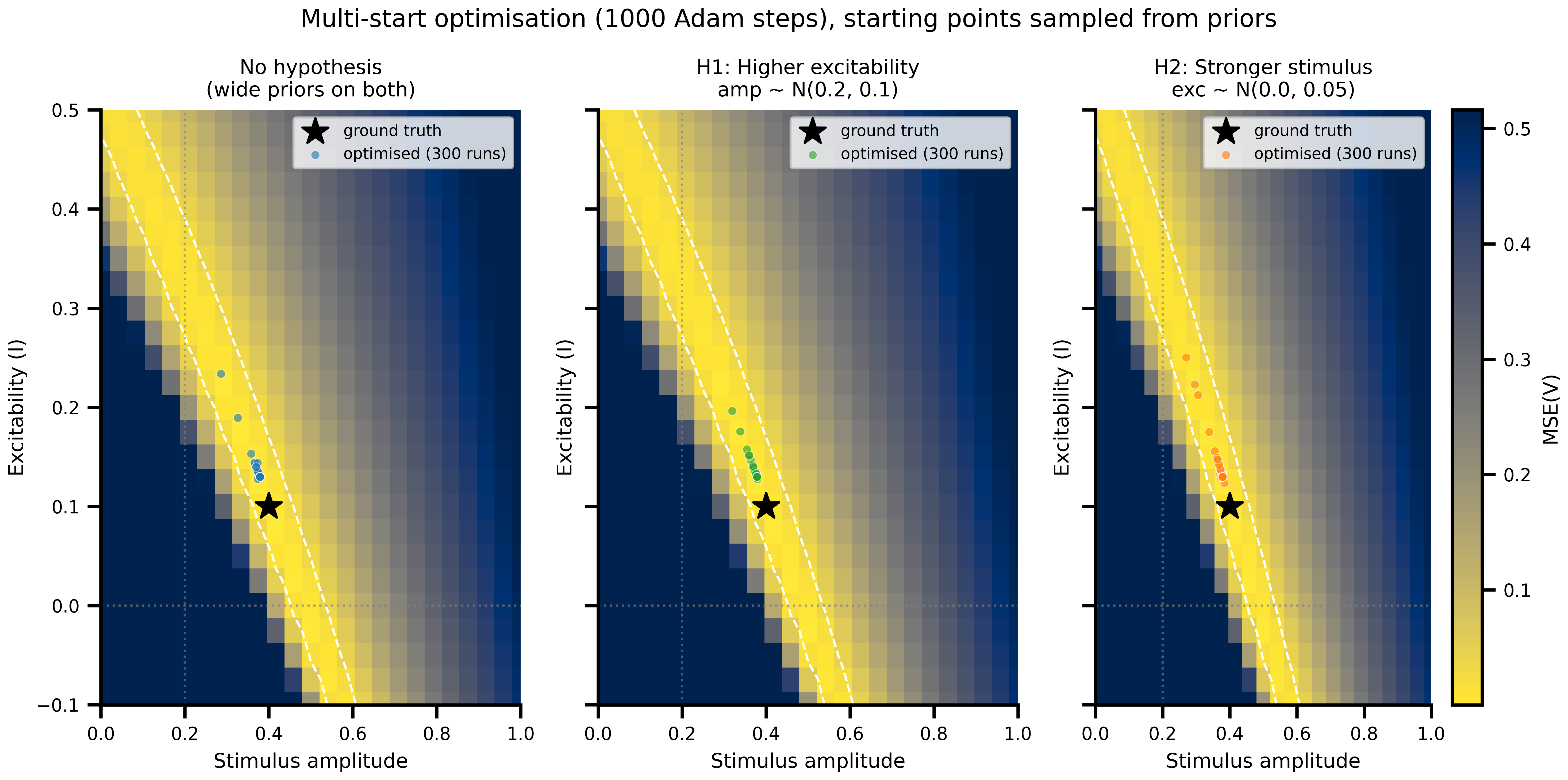
```{python}
#| label: fig-multistart
#| fig-cap: "**Multi-start optimization endpoints.** Each coloured dot is the final `(amp, I)` of one gradient-descent run. Endpoints cluster onto narrow regions of the ridge, but those regions just track where the starting points (sampled from the prior) happened to lie. The clustering is not a posterior. It is a smeared-out projection of the prior, with no notion of uncertainty attached."
#| code-fold: true
#| code-summary: "Show plotting code"
fig, axes = plt.subplots(1, 3, figsize=(10, 5), sharey=True)
for ax, key, color in zip(axes, SCENARIO_KEYS, COLORS):
pcm = _draw_landscape(ax)
ax.scatter(opt_results[key]["amplitude"], opt_results[key]["excitability"],
s=15, alpha=0.6, color=color, edgecolors="white", linewidths=0.3,
zorder=5, label=f"optimised ({N_SAMPLES} runs)")
ax.axvline(PRIOR_AMP_MEAN, color="gray", ls=":", lw=1.0, alpha=0.6)
ax.axhline(PRIOR_EXC_MEAN, color="gray", ls=":", lw=1.0, alpha=0.6)
ax.set_title(SCENARIO_LABELS[key], fontsize=9)
ax.legend(fontsize=7)
axes[0].set_ylabel("Excitability (I)")
fig.colorbar(pcm, ax=axes[-1], label="MSE(V)")
fig.suptitle(
f"Multi-start optimisation ({N_OPTIM_STEPS} Adam steps), starting points sampled from priors",
fontsize=11,
)
fig.tight_layout()
```
```{python}
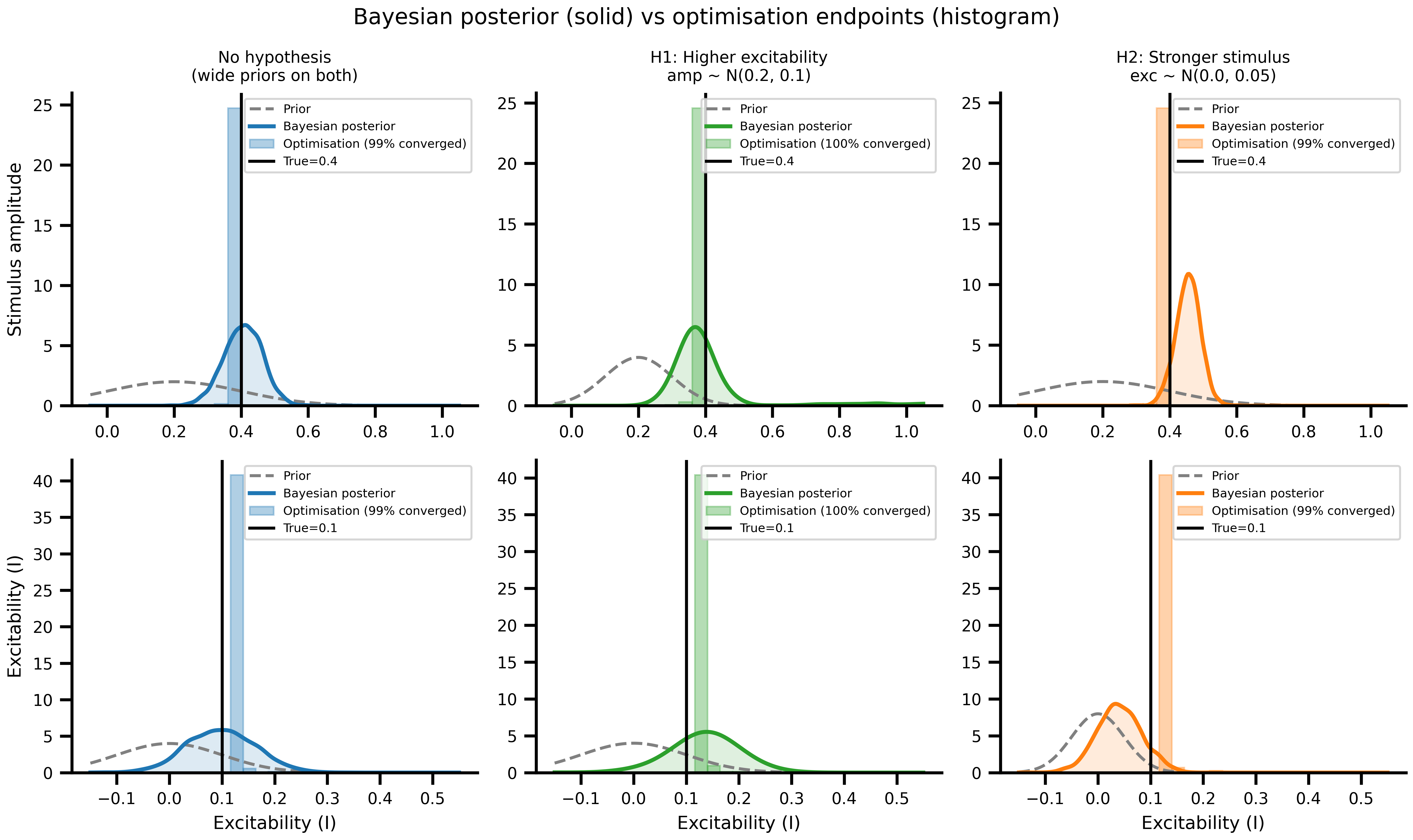
#| label: fig-bayes-vs-optim
#| fig-cap: "**Bayesian posteriors vs optimization endpoints, side by side.** Solid lines: Bayesian posterior densities. Translucent histograms: optimization endpoints from the same priors. The two are answers to different questions. Optimization tells you where the loss is low given a starting bias. Bayes tells you what to believe about the parameter given the data and a prior."
#| code-fold: true
#| code-summary: "Show plotting code"
# Filter optimisation results to landscape range (converged runs only)
amp_range = (float(amp_vals.min()), float(amp_vals.max()))
exc_range = (float(excit_vals.min()), float(excit_vals.max()))
opt_converged = {}
for key in SCENARIO_KEYS:
amp = opt_results[key]["amplitude"]
exc = opt_results[key]["excitability"]
mask = (
(amp >= amp_range[0]) & (amp <= amp_range[1]) &
(exc >= exc_range[0]) & (exc <= exc_range[1])
)
opt_converged[key] = {
"amplitude": amp[mask],
"excitability": exc[mask],
"pct": float(mask.sum()) / len(mask) * 100,
}
fig, axes = plt.subplots(2, 3, figsize=(10, 6), sharex="row")
param_meta_cmp = [
("amplitude", TRUE_AMPLITUDE, "Stimulus amplitude",
[dist.Normal(PRIOR_AMP_MEAN, PRIOR_AMP_STD[k]) for k in SCENARIO_KEYS],
amp_range),
("excitability", TRUE_EXCITABILITY, "Excitability (I)",
[dist.Normal(PRIOR_EXC_MEAN, PRIOR_EXC_STD[k]) for k in SCENARIO_KEYS],
exc_range),
]
for row, (param, true_val, xlabel, priors, hist_range) in enumerate(param_meta_cmp):
x = jnp.linspace(hist_range[0] - 0.05, hist_range[1] + 0.05, 300)
for col, (samples, key, prior, color) in enumerate(
zip(all_samples, SCENARIO_KEYS, priors, COLORS)
):
ax = axes[row, col]
kde_bayes = gaussian_kde(samples[param])
opt_vals = opt_converged[key][param]
ax.plot(x, jnp.exp(prior.log_prob(x)), color="gray", ls="--", lw=1.5, label="Prior")
ax.plot(x, kde_bayes(x), color=color, lw=2, label="Bayesian posterior")
ax.fill_between(x, kde_bayes(x), alpha=0.15, color=color)
if len(opt_vals) >= 1:
ax.hist(opt_vals, bins=25, range=hist_range, density=True,
color=color, alpha=0.35, edgecolor=color, linewidth=0.8,
label=f"Optimisation ({opt_converged[key]['pct']:.0f}% converged)")
ax.axvline(true_val, color="k", lw=1.5, label=f"True={true_val}")
if row == 0:
ax.set_title(SCENARIO_LABELS[key], fontsize=8)
if col == 0:
ax.set_ylabel(xlabel, fontsize=9)
if row == 1:
ax.set_xlabel(xlabel, fontsize=9)
ax.legend(fontsize=6)
fig.suptitle("Bayesian posterior (solid) vs optimisation endpoints (histogram)", fontsize=11)
fig.tight_layout()
```
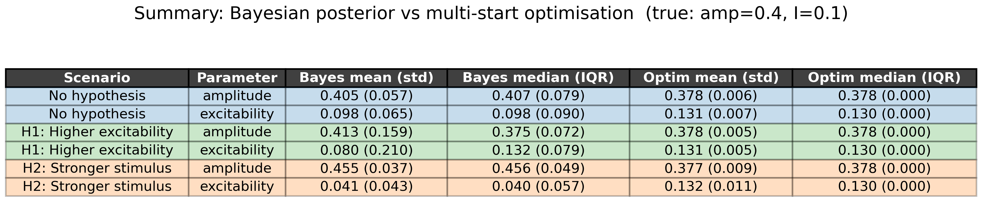
## Summary Table
The per-scenario numbers in one place. For each parameter and each scenario: mean and std, median and IQR, computed once from the Bayesian posterior and once from the multi-start optimization endpoints.
```{python}
#| label: fig-summary-table
#| fig-cap: "**Summary statistics by scenario and method.** For each scenario (A/B/C) and each parameter (amplitude, excitability), we report mean ± std and median ± IQR for the Bayesian posterior and for the multi-start optimization endpoints. Compare across rows to see how the same observation produces different inferences under different hypotheses."
#| code-fold: true
#| code-summary: "Show plotting code"
SHORT_NAMES = {"A": "No hypothesis", "B": "H1: Higher excitability", "C": "H2: Stronger stimulus"}
col_headers = [
"Scenario", "Parameter",
"Bayes mean (std)", "Bayes median (IQR)",
"Optim mean (std)", "Optim median (IQR)",
]
rows = []
for key, samples in zip(SCENARIO_KEYS, all_samples):
for param in ["amplitude", "excitability"]:
bayes_s = np.array(samples[param])
opt_s = np.array(opt_converged[key][param])
has_opt = len(opt_s) > 0
rows.append([
SHORT_NAMES[key], param,
f"{np.mean(bayes_s):.3f} ({np.std(bayes_s):.3f})",
f"{np.median(bayes_s):.3f} ({iqr(bayes_s):.3f})",
f"{np.mean(opt_s):.3f} ({np.std(opt_s):.3f})" if has_opt else "—",
f"{np.median(opt_s):.3f} ({iqr(opt_s):.3f})" if has_opt else "—",
])
fig, ax = plt.subplots(figsize=(8, 2), dpi=200)
ax.axis("off")
tbl = ax.table(cellText=rows, colLabels=col_headers, loc="center", cellLoc="center")
tbl.auto_set_font_size(False)
tbl.set_fontsize(8.5)
tbl.auto_set_column_width(col=list(range(len(col_headers))))
for (r, c), cell in tbl.get_celld().items():
if r == 0:
cell.set_facecolor("#404040")
cell.set_text_props(color="white", fontweight="bold")
elif r > 0:
color = COLORS[(r - 1) // 2]
cell.set_facecolor(color)
cell.set_alpha(0.25)
fig.suptitle("Summary: Bayesian posterior vs multi-start optimisation (true: amp=0.4, I=0.1)",
fontsize=11)
fig.tight_layout()
```
## When HMC stops being the right tool
Two parameters is the easy case. The harder question is what happens when the posterior lives in hundreds or thousands of dimensions, as it does for the connectivity-scale optimisation in the main paper.
**What scales.** The forward model is a JAX function, so one gradient call costs one forward plus one reverse-mode pass, almost independently of how many parameters the gradient is taken with respect to. For moderate parameter counts (roughly 10 to a few hundred) HMC with `dense_mass=True` works well, and the integration above is the template.
**What does not scale.** A dense mass matrix is `O(d²)` to store and learn, the warm-up cost grows with it, and multimodality compounds as the dimension rises. The cost per leapfrog step is the forward-model cost, which is fine here but painful for a long BOLD pipeline. For `N = 14,028` parameters, vanilla NUTS is not the answer.
**What is the answer at that scale.** Three alternatives stay inside the same differentiable workflow:
1. **Variational inference**: replace the posterior with a parametric family and minimise a KL objective using the same gradients. JAX-friendly; numpyro has `SVI` built in.
2. **Simulation-based inference**: train a density estimator on `(parameters, summary statistic)` pairs sampled from the prior and the simulator. Discussed below.
3. **Population-based search**: pymoo + JAX gives multi-objective Pareto fronts using the same `ParallelExecution` backbone, without leaving the JAX toolchain. Useful when uncertainty quantification is less important than exploring competing objectives.
## Off-ramp: simulation-based inference
SBI sidesteps the likelihood entirely. Sample parameters from a prior, run the simulator on each, summarise the output, and train a neural density estimator on those `(theta, x)` pairs. The trained network is a posterior conditioned on any observed summary. This trades the explicit likelihood for a learned inverse map, which is exactly the trade you want when the forward model is expensive, the likelihood is hard to write down, or the parameter count is large.
The integration with `tvboptim` is short because the simulator side is already done: `ParallelExecution` over `DataAxis` is the batched simulator that SBI needs. The sketch below shows the shape of the wiring (display only, not executed in this notebook):
```python
import torch
from sbi.inference import SNPE
from sbi.utils import BoxUniform

# 1. Prior in torch — sbi requires torch distributions
prior = BoxUniform(low=torch.tensor([0.0, -0.3]),
                   high=torch.tensor([1.0,  0.6]))
theta = prior.sample((N_SIM,))  # (N_SIM, 2)

# 2. Forward sims on the JAX side via ParallelExecution
net = build_network(TRUE_AMPLITUDE, TRUE_EXCITABILITY)
sf, cfg = prepare(net, Heun(), t0=0.0, t1=T1, dt=DT)
cfg.external.stimulus.amplitude = DataAxis(jnp.asarray(theta[:, 0]))
cfg.dynamics.I                  = DataAxis(jnp.asarray(theta[:, 1]))
sims = ParallelExecution(
    model=lambda c: summary_stats(sf(c).ys[obs_idx, 0, 0]),
    space=Space(cfg, mode="zip"),
    n_pmap=N_DEVICES, n_vmap=N_SIM // N_DEVICES,
).run()

# 3. Hand back to sbi to train a posterior estimator
x = torch.as_tensor(np.asarray(sims))
posterior = SNPE(prior=prior).append_simulations(theta, x).train()
samples = posterior.sample((4000,), x=torch.as_tensor(np.asarray(v_obs_summary)))
```
Trade-offs:
- **What this buys.** It scales to high-dim, accepts non-differentiable summaries, needs no closed-form likelihood, and reuses the same parallel forward model. The summary statistic can be any reduction: peak amplitude, FCD entries, BOLD KS distance.
- **What it costs.** `torch` becomes a runtime dependency, the JAX↔torch boundary is a numpy hop, and the training step lives outside the inference loop. On multi-GPU JAX setups the combined toolchain is fragile, which is why `tvboptim` does not vendor it.
- **When to skip SBI entirely.** For multi-objective optimisation without Bayesian uncertainty, pymoo on top of `ParallelExecution` gives Pareto fronts using the JAX toolchain alone. That is often enough when the question is "which parameter regimes satisfy which objectives" rather than "what is the posterior".
::: {.callout-note}
## Takeaways
- The forward model is **degenerate**: a ridge of `(amplitude, excitability)` pairs produces near-identical observations.
- **Optimization** collapses that ridge to a single arbitrary point. It is silent about residual uncertainty.
- **Bayesian inference** returns the full posterior along the ridge. The prior is where mechanistic evidence (a PET scan, a stimulator log) enters in a way the optimizer cannot represent.
- All three scenarios fit the data equally well. They differ only in which mechanistic explanation they prefer. That is the practical payoff of making priors explicit.
- The same ridge geometry appears whenever a forward model has internal trade-offs, including the effective-connectivity case where EI-tuning and Loss-based optimisation produce different solutions for the same data. The remedy there is the same as here: state the priors and report a posterior.
:::