PyRates Network Export

This example demonstrates creating a heterogeneous 3-node network in TVBO and running it via PyRates. We design a network where a slow oscillator drives two other nodes into opposite activity regimes, clearly visualizing the inter-node coupling.

Network Design

• Node 0 (Driver): Slow Hopf oscillator (~0.05 Hz) - acts as a pacemaker
• Node 1 (Excitable): FitzHugh-Nagumo in excitable regime - fires when driven above threshold
• Node 2 (Bistable): Modified oscillator - switches between low/high states

The driver provides excitatory input to Node 1 and inhibitory input to Node 2, causing anti-phase behavior.

Define Three Different Dynamics

from tvbo import Dynamics

# Slow Hopf oscillator - the DRIVER (~0.05 Hz period)
# Large amplitude, slow oscillation to clearly modulate other nodes
driver = Dynamics.from_string("""
name: SlowDriver
parameters:
  a:
    value: 0.5
  omega:
    value: 0.3
state_variables:
  x:
    equation:
      rhs: "a*x - omega*z - x*(x**2 + z**2) + c_in"
    initial_value: 1.0
  z:
    equation:
      rhs: "omega*x + a*z - z*(x**2 + z**2)"
    initial_value: 0.0
coupling_terms:
  c_in: {}
""")

# FitzHugh-Nagumo in EXCITABLE regime
# Will fire bursts when driven by positive input from driver
fhn = Dynamics.from_string("""
name: Excitable
parameters:
  a:
    value: 0.7
  b:
    value: 0.8
  tau:
    value: 12.5
  I_ext:
    value: 0.3
state_variables:
  v:
    equation:
      rhs: "v - v**3/3 - w + I_ext + c_in"
    initial_value: -1.0
  w:
    equation:
      rhs: "(v + a - b*w)/tau"
    initial_value: -0.5
coupling_terms:
  c_in: {}
""")

# Van der Pol as relaxation oscillator
# Receives INHIBITORY input - active when driver is LOW
vdp = Dynamics.from_string("""
name: Relaxation
parameters:
  mu:
    value: 2.0
state_variables:
  x:
    equation:
      rhs: "mu*(x - x**3/3 - w) + c_in"
    initial_value: -1.5
  w:
    equation:
      rhs: "x/mu"
    initial_value: 0.0
coupling_terms:
  c_in: {}
""")

Create SimulationExperiment with Network

import yaml
from tvbo import SimulationExperiment
from tvbo import Network

# Network topology:
# - Driver (node 0) sends POSITIVE coupling to Excitable (node 1)
# - Driver (node 0) sends NEGATIVE coupling to Relaxation (node 2)
# - This creates anti-phase modulation: when driver is UP, node 1 is excited, node 2 is suppressed

network_yaml = """
label: HeterogeneousModulation
number_of_nodes: 3
nodes:
  - id: 0
    label: Driver
    dynamics: SlowDriver
  - id: 1
    label: Excitable
    dynamics: Excitable
  - id: 2
    label: Relaxation
    dynamics: Relaxation
edges:
  - source: 0
    target: 1
    parameters:
      - weight:
          value: 0.8
    source_var: x_out
    target_var: c_in
  - source: 0
    target: 2
    parameters:
      weight:
        value: -0.6
    source_var: x_out
    target_var: c_in
  - source: 1
    target: 2
    parameters:
      - weight:
          value: 0.1
    source_var: v_out
    target_var: c_in
  - source: 2
    target: 1
    parameters:
      - weight:
          value: 0.1
    source_var: x_out
    target_var: c_in
"""

# Parse network from YAML
network = Network.from_string(network_yaml)

# Create experiment with dynamics library and network
exp = SimulationExperiment(
    dynamics={
        "SlowDriver": driver,
        "Excitable": fhn,
        "Relaxation": vdp,
    },
    network=network,
)

print(f"Network: {network.label}")
print(f"  Nodes: {[(n.id, n.label, n.dynamics) for n in network.nodes]}")
print(f"  Edges:")
for source, target, data in network.graph.edges(data=True):
    print(f"    {source} → {target}: {data['weight']}")

Network: HeterogeneousModulation
  Nodes: [(0, 'Driver', 'SlowDriver'), (1, 'Excitable', 'Excitable'), (2, 'Relaxation', 'Relaxation')]
  Edges:
    0 → 1: 0.8
    0 → 2: -0.6
    1 → 0: 0.8
    1 → 2: 0.1
    1 → 2: 0.1
    2 → 0: -0.6
    2 → 1: 0.1
    2 → 1: 0.1

Export to PyRates YAML

The streamlined API exports directly via SimulationExperiment.to_yaml(format="pyrates"):

# Provide minimal integration settings required by the schema
exp.integration.duration = 200.0
exp.integration.step_size = 0.01
yaml_content = exp.to_yaml(format="pyrates")

print("=== Generated PyRates YAML ===")
print(yaml_content)

=== Generated PyRates YAML ===

%YAML 1.2
---
# PyRates Experiment Template
# Generated from TVBO Network
# This file is self-contained and ready for PyRates simulation.

# OPERATORS (Model Dynamics)


SlowDriver_op:
  base: OperatorTemplate
  description: "SlowDriver"
  equations:
    - "x' = c_in + a*x - omega*z - x*(x**2 + z**2)"
    - "z' = a*z + omega*x - z*(x**2 + z**2)"
  variables:
    x: variable(1.0)
    z: variable(0.0)
    a: 0.5
    omega: 0.3
    c_in: input



Excitable_op:
  base: OperatorTemplate
  description: "Excitable"
  equations:
    - "v' = I_ext + c_in + v - w - v**3/3"
    - "w' = (a + v - b*w)/tau"
  variables:
    v: variable(-1.0)
    w: variable(-0.5)
    a: 0.7
    b: 0.8
    tau: 12.5
    I_ext: 0.3
    c_in: input



Relaxation_op:
  base: OperatorTemplate
  description: "Relaxation"
  equations:
    - "x' = c_in + mu*(x - w - x**3/3)"
    - "w' = x/mu"
  variables:
    x: variable(-1.5)
    w: variable(0.0)
    mu: 2.0
    c_in: input


# NODES (Network Topology)


Excitable:
  base: NodeTemplate
  operators:
    - Excitable_op

Relaxation:
  base: NodeTemplate
  operators:
    - Relaxation_op

SlowDriver:
  base: NodeTemplate
  operators:
    - SlowDriver_op

# CIRCUIT (Complete Network)

HeterogeneousModulation:
  base: CircuitTemplate
  nodes:
    Driver: SlowDriver
    Excitable: Excitable
    Relaxation: Relaxation
  edges:
    - [Driver/SlowDriver_op/x, Excitable/Excitable_op/c_in, null, {weight: 1.0, delay: 0.0}]
    - [Driver/SlowDriver_op/x, Relaxation/Relaxation_op/c_in, null, {weight: 1.0, delay: 0.0}]
    - [Excitable/Excitable_op/v, Relaxation/Relaxation_op/c_in, null, {weight: 1.0, delay: 0.0}]
    - [Relaxation/Relaxation_op/x, Excitable/Excitable_op/c_in, null, {weight: 1.0, delay: 0.0}]

# Run with PyRates backend - returns TVBO TimeSeries
exp.integration.duration = 300.0
exp.integration.step_size = 0.01

res = exp.run('pyrates')

Compilation Progress
--------------------
    (1) Translating the circuit template into a networkx graph representation...
        ...finished.
    (2) Preprocessing edge transmission operations...
        ...finished.
    (3) Parsing the model equations into a compute graph...
        ...finished.
    Model compilation was finished.
Simulation Progress
-------------------
     (1) Generating the network run function...
     (2) Processing output variables...
        ...finished.
     (3) Running the simulation...
        ...finished after 1.218634207998548s.

# Check the result format
print(res)
print(f"\nData shape: {res.data.shape}  →  (time, state_vars, nodes, modes)")

TimeSeries
├── time: f64[30000](numpy)
├── data: f32[30000,4,3,1](numpy)
├── labels_dimensions
│   ├── State Variable
│   │   ├── [0]: "x"
│   │   ├── [1]: "z"
│   │   ├── [2]: "v"
│   │   └── [3]: "w"
│   └── Region
│       ├── [0]: "Driver"
│       ├── [1]: "Excitable"
│       └── [2]: "Relaxation"
├── title: "TimeSeries"
├── network: NoneType
├── sample_period: 0.01
├── dt: 0.01
├── sample_period_unit: "ms"
├── units
│   ├── time: "ms"
│   ├── state: NoneType
│   ├── region: NoneType
│   └── mode: NoneType
└── labels_ordering
    ├── [0]: "Time"
    ├── [1]: "State Variable"
    ├── [2]: "Space"
    └── [3]: "Mode"

Data shape: (30000, 4, 3, 1)  →  (time, state_vars, nodes, modes)

res.get_region('Excitable').plot()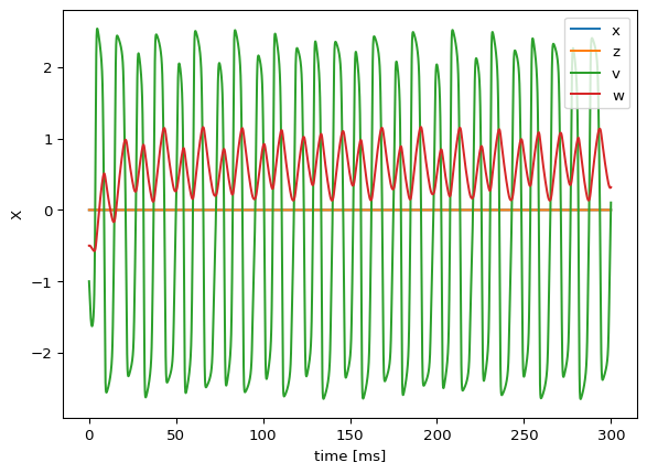

Run in PyRates

For manual control, you can still run PyRates directly:

import os
import shutil
from pyrates.frontend import CircuitTemplate
from pyrates import clear

# Write to temporary package
os.makedirs("_net", exist_ok=True)
open("_net/__init__.py", "w").close()
with open("_net/model.yaml", "w") as f:
    f.write(yaml_content)

# Load and simulate - longer time to see slow modulation
circuit = CircuitTemplate.from_yaml("_net.model.HeterogeneousModulation")
result = circuit.run(
    step_size=0.01,
    simulation_time=300.0,  # Longer to see multiple driver cycles
    outputs={
        "driver": "Driver/SlowDriver_op/x",
        "excitable": "Excitable/Excitable_op/v",
        "relaxation": "Relaxation/Relaxation_op/x",
    },
    solver="heun",
)
clear(circuit)
shutil.rmtree("_net")

print(f"Simulated {len(result)} time points over {result.index[-1]:.0f} ms")

Compilation Progress
--------------------
    (1) Translating the circuit template into a networkx graph representation...
        ...finished.
    (2) Preprocessing edge transmission operations...
        ...finished.
    (3) Parsing the model equations into a compute graph...
        ...finished.
    Model compilation was finished.
Simulation Progress
-------------------
     (1) Generating the network run function...
     (2) Processing output variables...
        ...finished.
     (3) Running the simulation...
        ...finished after 1.1086252500026603s.
Simulated 30000 time points over 300 ms

Visualize

import matplotlib.pyplot as plt
import numpy as np

fig, axes = plt.subplots(3, 1, figsize=(12, 8), sharex=True)

t = result.index
t_tvbo = res.time

# Plot Driver (slow oscillation)
ax = axes[0]
ax.plot(t, result["driver"], 'C0', lw=2, label="PyRates: Driver x")
# Overlay TVBO data with dashed line
driver_tvbo = res.get_region('Driver').get_state_variable('x')
ax.plot(t_tvbo, driver_tvbo.data[:, 0, 0, 0], 'k--', lw=1.5, alpha=0.7, label="TVBO TimeSeries")
ax.axhline(0, color='gray', ls='--', alpha=0.5)
ax.set_ylabel("Driver\n(Hopf)")
ax.legend(loc='upper right')
ax.set_title("Comparison: PyRates DataFrame vs TVBO TimeSeries", fontsize=12)

# Plot Excitable
ax = axes[1]
ax.plot(t, result["excitable"], 'C1', lw=2, label="PyRates: Excitable v")
excitable_tvbo = res.get_region('Excitable').get_state_variable('v')
ax.plot(t_tvbo, excitable_tvbo.data[:, 0, 0, 0], 'k--', lw=1.5, alpha=0.7, label="TVBO TimeSeries")
ax.axhline(0, color='gray', ls='--', alpha=0.5)
ax.set_ylabel("Excitable\n(FHN)")
ax.legend(loc='upper right')

# Plot Relaxation
ax = axes[2]
ax.plot(t, result["relaxation"], 'C2', lw=2, label="PyRates: Relaxation x")
relaxation_tvbo = res.get_region('Relaxation').get_state_variable('x')
ax.plot(t_tvbo, relaxation_tvbo.data[:, 0, 0, 0], 'k--', lw=1.5, alpha=0.7, label="TVBO TimeSeries")
ax.axhline(0, color='gray', ls='--', alpha=0.5)
ax.set_ylabel("Relaxation\n(VdP)")
ax.set_xlabel("Time (ms)")
ax.legend(loc='upper right')

plt.tight_layout()
plt.show()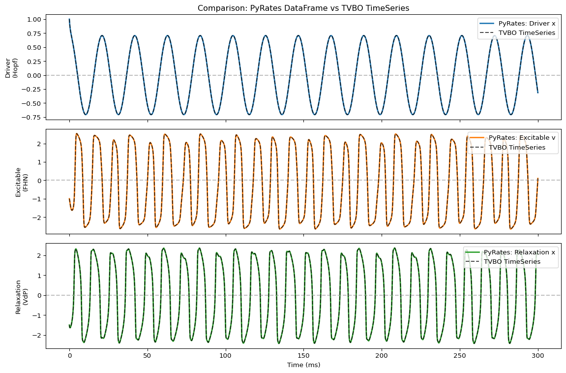

Phase Relationship Analysis

fig, ax = plt.subplots(figsize=(10, 4))

# Overlay all three normalized to similar scale
driver_norm = (result["driver"] - result["driver"].mean()) / result["driver"].std()
excitable_norm = (result["excitable"] - result["excitable"].mean()) / result["excitable"].std()
relaxation_norm = (result["relaxation"] - result["relaxation"].mean()) / result["relaxation"].std()

ax.plot(t, driver_norm, 'C0', lw=2, alpha=0.8, label="Driver (normalized)")
ax.plot(t, excitable_norm, 'C1', lw=1.5, alpha=0.8, label="Excitable (normalized)")
ax.plot(t, relaxation_norm, 'C2', lw=1.5, alpha=0.8, label="Relaxation (normalized)")

ax.set_xlabel("Time (ms)")
ax.set_ylabel("Normalized Activity")
ax.set_title("Phase Relationships: Excitable follows Driver, Relaxation is anti-phase")
ax.legend(loc='upper right')
ax.grid(True, alpha=0.3)

# Zoom to show phase relationship
ax.set_xlim(50, 200)

plt.tight_layout()
plt.show()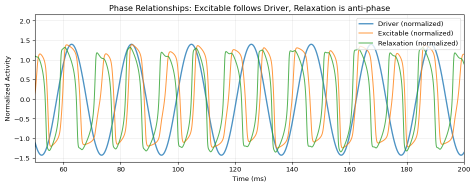

---

Use Case 2: Synaptic Plasticity

This section demonstrates how to model short-term synaptic plasticity using TVBO and PyRates. We implement the Tsodyks-Markram model which captures both synaptic depression and facilitation.

Network Architecture

The network models a single pre-synaptic neuron connecting to a post-synaptic neuron through three parallel synaptic pathways, each with different plasticity:

flowchart LR
    Pre["Pre-synaptic<br/>Neuron"]

    Dep["Depression<br/>Synapse"]
    Fac["Facilitation<br/>Synapse"]
    TM["Tsodyks-Markram<br/>Synapse"]

    Post["Post-synaptic<br/>Neuron"]

    Pre -->|"r_out"| Dep
    Pre -->|"r_out"| Fac
    Pre -->|"r_out"| TM

    Dep -->|"r_eff"| Post
    Fac -->|"r_eff"| Post
    TM -->|"r_eff"| Post

This allows direct comparison of how different plasticity mechanisms modulate transmission to the same post-synaptic target.

Synaptic Plasticity Models

Short-term synaptic plasticity modulates synaptic strength based on recent activity:

• Depression: Repeated stimulation depletes neurotransmitter resources
• Facilitation: Repeated stimulation increases release probability
• Tsodyks-Markram: Combines both effects with resource variable \(x\) and utilization \(u\)

Output Variables in PyRates

TVBO supports output variables with algebraic equations (e.g., r_eff = r_in * x). These are exported to PyRates as output-type variables. However, PyRates only allows monitoring state variables directly. Output variables are computed during simulation but cannot be accessed via the outputs parameter of circuit.run().

Solution: Monitor the underlying state variables and compute the output expressions post-hoc. This is demonstrated in this example.

Define Plasticity Dynamics

from tvbo import Dynamics

# Tsodyks-Markram sho#rt-term plasticity model
# Combines depression (x) and facilitation (u)
# r_eff is an output (algebraic equation) - PyRates renders this correctly
tsodyks = Dynamics.from_string("""
name: TsodyksMarkram
description: "Short-term synaptic plasticity with depression and facilitation"
parameters:
  tau_x:
    value: 200.0
    description: "Recovery time constant for depression (ms)"
  tau_u:
    value: 50.0
    description: "Recovery time constant for facilitation (ms)"
  U0:
    value: 0.2
    description: "Baseline release probability"
  k:
    value: 0.5
    description: "Depression rate"
  k_fac:
    value: 0.05
    description: "Facilitation rate"
state_variables:
  x:
    equation:
      rhs: "(1 - x)/tau_x - k*x*u*r_in"
    initial_value: 1.0
    description: "Available synaptic resources (depression variable)"
  u:
    equation:
      rhs: "(U0 - u)/tau_u + k_fac*(1 - u)*r_in"
    initial_value: 0.2
    description: "Release probability (facilitation variable)"
coupling_terms:
  r_in: {}
derived_variables:
  r_eff:
    equation:
      rhs: "r_in*x*u"
    description: "Effective synaptic transmission"
output:
    - r_eff
""")

# Pure synaptic depression model
depression = Dynamics.from_string("""
name: Depression
description: "Short-term synaptic depression only"
parameters:
  tau_x:
    value: 300.0
    description: "Recovery time constant (ms)"
  k:
    value: 0.3
    description: "Depression rate"
state_variables:
  x:
    equation:
      rhs: "(1 - x)/tau_x - k*x*r_in"
    initial_value: 1.0
    description: "Available synaptic resources"
coupling_terms:
  r_in: {}
derived_variables:
  r_eff:
    equation:
      rhs: "r_in*x"
    description: "Effective transmission with depression"
output:
    - r_eff
""")

# Pure synaptic facilitation model
facilitation = Dynamics.from_string("""
name: Facilitation
description: "Short-term synaptic facilitation only"
parameters:
  tau_u:
    value: 100.0
    description: "Recovery time constant (ms)"
  U0:
    value: 0.2
    description: "Baseline release probability"
  k_fac:
    value: 0.01
    description: "Facilitation rate"
state_variables:
  u:
    equation:
      rhs: "(U0 - u)/tau_u + k_fac*(1 - u)*r_in"
    initial_value: 0.2
    description: "Release probability"
coupling_terms:
  r_in: {}
derived_variables:
  r_eff:
    equation:
      rhs: "r_in*u"
    description: "Effective transmission with facilitation"
output:
 - r_eff
""")

# Simple rate neuron (I_ext=0.0, will receive external stimulus)
rate_neuron = Dynamics.from_string("""
name: RateNeuron
description: "Simple rate-based neuron with external input"
parameters:
  tau:
    value: 10.0
  I_ext:
    value: 0.0
state_variables:
  r:
    equation:
      rhs: "(-r + I_ext + r_in)/tau"
    initial_value: 0.0
coupling_terms:
  r_in: {}
""")

print(f"Created plasticity models: {tsodyks.name}, {depression.name}, {facilitation.name}")

Created plasticity models: TsodyksMarkram, Depression, Facilitation

Create Network with Plastic Synapses

import yaml
from tvbo import SimulationExperiment
from tvbo import Network

# Network: Pre-synaptic neuron → three parallel synaptic pathways → Post-synaptic neuron
# This allows direct comparison of how different plasticity affects the SAME post-synaptic target

network_yaml = """
label: SynapticPlasticityComparison
number_of_nodes: 5
nodes:
  - id: 0
    label: PreSynaptic
    dynamics: RateNeuron
  - id: 1
    label: DepressionSynapse
    dynamics: Depression
  - id: 2
    label: FacilitationSynapse
    dynamics: Facilitation
  - id: 3
    label: TsodyksSynapse
    dynamics: TsodyksMarkram
  - id: 4
    label: PostSynaptic
    dynamics: RateNeuron
edges:
  # Pre-synaptic drives all three synaptic relays
  - source: 0
    target: 1
    parameters:
        - weight:
            value: 1.0
    source_var: r_out
    target_var: r_in
  - source: 0
    target: 2
    parameters:
        - weight:
            value: 1.0
    source_var: r_out
    target_var: r_in
  - source: 0
    target: 3
    parameters:
        - weight:
            value: 1.0
    source_var: r_out
    target_var: r_in
  # All synapses converge onto the post-synaptic neuron
  - source: 1
    target: 4
    parameters:
        - weight:
            value: 0.33
    source_var: r_eff
    target_var: r_in
  - source: 2
    target: 4
    parameters:
        - weight:
            value: 0.33
    source_var: r_eff
    target_var: r_in
  - source: 3
    target: 4
    parameters:
        - weight:
            value: 0.33
    source_var: r_eff
    target_var: r_in
"""

# Parse network and create experiment with all components
network_plasticity = Network(**yaml.safe_load(network_yaml))

exp_plasticity = SimulationExperiment(
    dynamics={
        "RateNeuron": rate_neuron,
        "Depression": depression,
        "Facilitation": facilitation,
        "TsodyksMarkram": tsodyks,
    },
    network=network_plasticity,
)

print(f"Network: {network_plasticity.label}")
print("Nodes:")
for n in network_plasticity.nodes:
    print(f"  {n.id}: {n.label} ({n.dynamics})")
print("Edges:")
for source, target, data in network_plasticity.graph.edges(data=True):
    print(f"  {source} → {target} (w={data['weight']})")

Network: SynapticPlasticityComparison
Nodes:
  0: PreSynaptic (RateNeuron)
  1: DepressionSynapse (Depression)
  2: FacilitationSynapse (Facilitation)
  3: TsodyksSynapse (TsodyksMarkram)
  4: PostSynaptic (RateNeuron)
Edges:
  0 → 1 (w=1.0)
  0 → 2 (w=1.0)
  0 → 3 (w=1.0)
  1 → 0 (w=1.0)
  1 → 4 (w=0.33)
  2 → 0 (w=1.0)
  2 → 4 (w=0.33)
  3 → 0 (w=1.0)
  3 → 4 (w=0.33)
  4 → 1 (w=0.33)
  4 → 2 (w=0.33)
  4 → 3 (w=0.33)

Export and Run

import os
import shutil
from pyrates.frontend import CircuitTemplate
from pyrates import clear
import numpy as np

# Export using streamlined API
yaml_plasticity = exp_plasticity.to_yaml(format="pyrates")

# Write to temporary package
os.makedirs("_plasticity", exist_ok=True)
open("_plasticity/__init__.py", "w").close()
with open("_plasticity/model.yaml", "w") as f:
    f.write(yaml_plasticity)

# Create pulsed input signal (bursts of activity)
T = 500.0
dt = 0.1
time = np.arange(0, T, dt)

# Create burst pattern: pulses at regular intervals
pulse_times = [50, 100, 150, 200, 250, 350, 400, 450]
input_signal = np.zeros_like(time)
for pt in pulse_times:
    # Each pulse is a brief 10ms square wave
    mask = (time >= pt) & (time < pt + 10)
    input_signal[mask] = 5.0

# Load and simulate
# Note: PyRates output variables (algebraic equations) cannot be monitored directly.
# We monitor state variables and compute outputs post-hoc.
circuit = CircuitTemplate.from_yaml("_plasticity.model.SynapticPlasticityComparison")
result_plasticity = circuit.run(
    step_size=dt,
    simulation_time=T,
    inputs={"PreSynaptic/RateNeuron_op/I_ext": input_signal},
    outputs={
        "pre": "PreSynaptic/RateNeuron_op/r",
        "depression_x": "DepressionSynapse/Depression_op/x",
        "facilitation_u": "FacilitationSynapse/Facilitation_op/u",
        "tsodyks_x": "TsodyksSynapse/TsodyksMarkram_op/x",
        "tsodyks_u": "TsodyksSynapse/TsodyksMarkram_op/u",
        "post": "PostSynaptic/RateNeuron_op/r",
    },
    solver="heun",
)
clear(circuit)
shutil.rmtree("_plasticity")

# Compute output variables (r_eff = r_in * state) post-hoc
# Since edges have weight=1.0 to synapses, r_in equals the source r_out
result_plasticity["depression_out"] = result_plasticity["pre"] * result_plasticity["depression_x"]
result_plasticity["facilitation_out"] = result_plasticity["pre"] * result_plasticity["facilitation_u"]
result_plasticity["tsodyks_out"] = result_plasticity["pre"] * result_plasticity["tsodyks_x"] * result_plasticity["tsodyks_u"]

print(f"Simulated {len(result_plasticity)} time points")

Compilation Progress
--------------------
    (1) Translating the circuit template into a networkx graph representation...
        ...finished.
    (2) Preprocessing edge transmission operations...
        ...finished.
    (3) Parsing the model equations into a compute graph...
        ...finished.
    Model compilation was finished.
Simulation Progress
-------------------
     (1) Generating the network run function...
     (2) Processing output variables...
        ...finished.
     (3) Running the simulation...
        ...finished after 0.2515613329996995s.
Simulated 5000 time points

Visualize Plasticity Effects

import matplotlib.pyplot as plt

fig, axes = plt.subplots(5, 1, figsize=(12, 12), sharex=True)
t = result_plasticity.index

# Pre-synaptic input signal
ax = axes[0]
ax.plot(t, result_plasticity["pre"], 'k', lw=2, label="Pre-synaptic Rate")
ax.set_ylabel("Pre-synaptic\nRate")
ax.set_title("Short-Term Synaptic Plasticity: Pre → Synapse → Post", fontsize=12)
ax.legend(loc='upper right')
ax.set_ylim(-0.5, 6)

# Depression: resources decrease with repeated stimulation
ax = axes[1]
ax.plot(t, result_plasticity["depression_x"], 'C0', lw=2, label="Resources (x)")
ax.plot(t, result_plasticity["depression_out"], 'C0--', lw=1.5, alpha=0.7, label="Synaptic output")
ax.set_ylabel("Depression")
ax.legend(loc='upper right')
ax.axhline(1.0, color='gray', ls=':', alpha=0.5)
ax.annotate("Resources deplete →", xy=(150, 0.5), fontsize=9, color='C0')

# Facilitation: release probability increases with repeated stimulation
ax = axes[2]
ax.plot(t, result_plasticity["facilitation_u"], 'C1', lw=2, label="Release prob (u)")
ax.plot(t, result_plasticity["facilitation_out"], 'C1--', lw=1.5, alpha=0.7, label="Synaptic output")
ax.set_ylabel("Facilitation")
ax.legend(loc='upper right')
ax.annotate("← Release prob increases", xy=(150, 0.6), fontsize=9, color='C1')

# Tsodyks-Markram: combined effect
ax = axes[3]
ax.plot(t, result_plasticity["tsodyks_x"], 'C2', lw=2, label="Resources (x)")
ax.plot(t, result_plasticity["tsodyks_u"], 'C3', lw=2, label="Release prob (u)")
ax.plot(t, result_plasticity["tsodyks_out"], 'k--', lw=1.5, alpha=0.7, label="Synaptic output (x·u·r)")
ax.set_ylabel("Tsodyks-\nMarkram")
ax.legend(loc='upper right')
ax.annotate("Combined: initial facilitation then depression", xy=(200, 0.3), fontsize=9)

# Post-synaptic response (receives summed input from all three synapses)
ax = axes[4]
ax.plot(t, result_plasticity["post"], 'C4', lw=2, label="Post-synaptic Rate")
ax.set_ylabel("Post-synaptic\nRate")
ax.set_xlabel("Time (ms)")
ax.legend(loc='upper right')
ax.annotate("Receives summed plastic inputs", xy=(200, 0.5), fontsize=9, color='C4')

plt.tight_layout()
plt.show()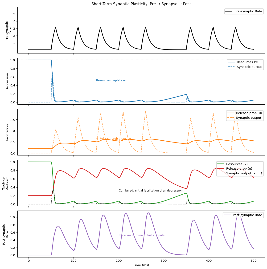

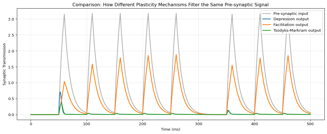
Compare Synaptic Outputs

fig, ax = plt.subplots(figsize=(12, 5))

ax.plot(t, result_plasticity["pre"], 'k', lw=2, alpha=0.3, label="Pre-synaptic input")
ax.plot(t, result_plasticity["depression_out"], 'C0', lw=2, label="Depression output")
ax.plot(t, result_plasticity["facilitation_out"], 'C1', lw=2, label="Facilitation output")
ax.plot(t, result_plasticity["tsodyks_out"], 'C2', lw=2, label="Tsodyks-Markram output")

ax.set_xlabel("Time (ms)")
ax.set_ylabel("Synaptic Transmission")
ax.set_title("Comparison: How Different Plasticity Mechanisms Filter the Same Pre-synaptic Signal")
ax.legend(loc='upper right')
ax.grid(True, alpha=0.3)

plt.tight_layout()
plt.show()