A pulse stimulus is delivered to a Generic2dOscillator and we record a noisy time series. From that one recording, we want to recover two things: how strong the stimulus was, and how excitable the underlying system is. The problem is that these two parameters trade off. A weaker stimulus into a more excitable system produces almost the same trajectory as a stronger stimulus into a less excitable one.
Gradient descent picks an arbitrary point on this ridge of equally good fits and reports it as the answer. Bayesian inference reports the whole ridge, and lets prior knowledge about either parameter (a device log, a PET scan) narrow it down in a principled way.
The notebook proceeds in four steps:
Generate a noisy observation from a known ground truth.
Scan the MSE landscape and show that many parameter pairs explain the data.
Sample three posteriors with different priors on the same observation.
Compare those posteriors against multi-start gradient descent on the same priors.
What you’ll learn
Concepts: what parameter degeneracy looks like, why a point estimate hides it, and how a prior turns “any answer on the ridge” into “the answer consistent with what you already know”.
TVB-Optim idioms: wiring tvboptim forward simulation into a numpyro model, using GridAxis for landscape scans, DataAxis to batch posterior-predictive draws.
Workflow: what changes when you swap an optimizer for a sampler, and how to read the result.
Environment Setup and Imports
# Set up environment — XLA_FLAGS must be set BEFORE importing jax. Here we expose# 25 virtual devices so ParallelExecution can spread landscape scans, posterior# predictive draws, and multi-start optimisations across many devices at once.import osN_DEVICES =25os.environ["XLA_FLAGS"] =f"--xla_force_host_platform_device_count={N_DEVICES}"import numpy as npimport jaximport jax.numpy as jnpimport matplotlib.pyplot as pltimport numpyroimport numpyro.distributions as distimport optaxfrom numpyro.infer import MCMC, NUTSfrom numpyro.infer.util import log_densityfrom scipy.stats import gaussian_kde, iqrfrom tvboptim.execution import ParallelExecutionfrom tvboptim.experimental.network_dynamics import Network, prepare, solve as nd_solvefrom tvboptim.experimental.network_dynamics.dynamics.tvb import Generic2dOscillatorfrom tvboptim.experimental.network_dynamics.coupling import LinearCouplingfrom tvboptim.experimental.network_dynamics.graph import DenseGraphfrom tvboptim.experimental.network_dynamics.external_input import PulseInputfrom tvboptim.experimental.network_dynamics.solvers import Heunfrom tvboptim.types import DataAxis, GridAxis, Space, Parameter, collect_parametersfrom tvboptim.optim import OptaxOptimizerfrom tvboptim.utils import set_cache_path, cache# Cache directory for expensive MCMC and optimisation runsset_cache_path("./bayes_stim")
2 Shared Settings and Priors
The three scenarios use identical prior means and differ only in their standard deviations. A tight prior on one parameter is how we tell the model that we already have evidence about it:
A: no hypothesis. Wide priors on both parameters.
B (H1, higher excitability): tight prior on amplitude. The stimulator log is trusted, so the data has to be explained via excitability.
C (H2, stronger stimulus): tight prior on excitability. PET or gene-expression evidence pins excitability down, so the data has to be explained via amplitude.
T1 =150.0DT =0.2ONSET =10.0DURATION =1.0TRUE_AMPLITUDE =0.4TRUE_EXCITABILITY =0.1OBS_NOISE_SIGMA =0.1# data generation noiseLIKELIHOOD_SIGMA =0.2# fixed in likelihood — intentionally flat along ridge so priors steerPRIOR_AMP_MEAN =0.2PRIOR_EXC_MEAN =0.0# Scenario priors: all share the same means; hypotheses constrain one parameter (tight σ).# Standard deviations: No hyp. H1 H2PRIOR_AMP_STD = {"A": 0.2, "B": 0.1, "C": 0.2} # H1: tight amp → excitability explainsPRIOR_EXC_STD = {"A": 0.1, "B": 0.1, "C": 0.05} # H2: tight exc → stimulus explainsSCENARIO_LABELS = {"A": "No hypothesis\n(wide priors on both)","B": f"H1: Higher excitability\namp ~ N({PRIOR_AMP_MEAN}, {PRIOR_AMP_STD['B']})","C": f"H2: Stronger stimulus\nexc ~ N({PRIOR_EXC_MEAN}, {PRIOR_EXC_STD['C']})",}DYNAMICS_PARAMS =dict(a=-1.5, b=-15.0, c=0.0, d=0.015, e=3.0, f=1.0, tau=4.0)weights = jnp.zeros((1, 1))SCENARIO_KEYS = ["A", "B", "C"]COLORS = ["tab:blue", "tab:green", "tab:orange"]
3 Stimulation in TVB-Optim — quick recap
The stimulus in this notebook is a rectangular pulse delivered to a single-node Generic2dOscillator. In TVB-Optim, stimuli live in the external_input slot of a Network and are routed by name. The dynamics class declares which names it accepts via its EXTERNAL_INPUTS attribute; for Generic2dOscillator the name is 'stimulus', and the value gets added into the equation for the fast variable V.
The pulse itself is a PulseInput parametrized by three numbers:
onset — when the pulse starts (ms).
duration — how long it stays on.
amplitude — the constant value driving V during the on-window.
PulseInput is a parametric input: a function of time that the solver evaluates at each step. The alternative is DataInput, which interpolates between recorded samples — useful when you have an experimental stimulator trace rather than an idealized waveform. Any parameter of an external input can be wrapped in Parameter(...) to mark it as optimizable, which is exactly what we do later when comparing Bayesian inference against gradient descent.
In code, the wiring lives inside build_network (in the collapsed helpers block below):
The name "stimulus" on the left of the dict has to match the name in EXTERNAL_INPUTS. The two free parameters of this notebook — amplitude (a property of the input) and I (a property of the dynamics, the excitability) — sit in different parts of the config, but the Bayesian model treats them symmetrically.
4 The Bayesian Model
This is the conceptual core of the notebook, so we look at it on its own. make_model returns a numpyro model that describes the joint distribution of parameters and data. Three things happen inside the inner model function:
Priors.numpyro.sample("amplitude", dist.Normal(...)) draws an amplitude from the prior. It also tells numpyro: this is a latent variable named “amplitude”, track its log-density. Same for excitability. The standard deviations amp_std and exc_std are scenario-specific and baked in from the closure.
Forward simulation. The sampled parameters are written into the simulation config and the forward model produces a predicted trajectory v_pred.
Likelihood. The final numpyro.sample("obs", ..., obs=v_obs) declares that the observation v_obs is a noisy version of v_pred with fixed noise scale LIKELIHOOD_SIGMA. The obs= keyword is what turns this from “sample obs” into “score obs against the model”.
def make_model(scenario_key):"""Return a numpyro model with scenario-specific prior widths baked in as closure constants.""" amp_std =float(PRIOR_AMP_STD[scenario_key]) exc_std =float(PRIOR_EXC_STD[scenario_key])def model(v_obs, solve_fn, config, obs_idx):# 1. Priors on the two latent parameters amplitude = numpyro.sample("amplitude", dist.Normal(PRIOR_AMP_MEAN, amp_std)) excitability = numpyro.sample("excitability", dist.Normal(PRIOR_EXC_MEAN, exc_std))# 2. Forward simulation with the sampled parameters config.external.stimulus.amplitude = amplitude config.dynamics.I = excitability v_pred = solve_fn(config).ys[obs_idx, 0, 0]# 3. Likelihood: observation is v_pred + Gaussian noise numpyro.sample("obs", dist.Normal(v_pred, LIKELIHOOD_SIGMA), obs=v_obs)return model
NUTS then samples the joint posterior over amplitude and excitability by combining (1), (2), and (3). The sampler never sees the priors as Python objects: it only sees the resulting log-density. That is why amp_std and exc_std are converted to Python floats before being captured in the closure. Passing live dist.Normal objects in from the outside would break JIT tracing and silently drop the priors.
Other helpers (network, loss, MCMC runner, plotting)
These are plumbing — the network factory, the MSE loss for the optimization comparison, the MCMC runner with NUTS settings, and a small landscape-drawing helper used by several figures.
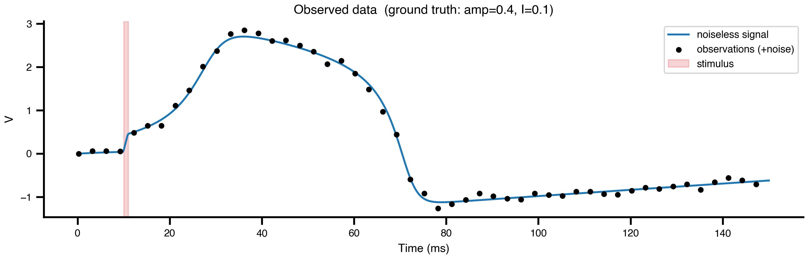
Simulate the forward model at the true parameters, subsample every 15 steps, add Gaussian noise. The noiseless trajectory is kept around as the reference for MSE in the landscape scan that follows.
# Noiseless signal as base ensures MLE at true params. Ridge points produce near-identical# noiseless signals, so the likelihood is flat along the ridge and priors steer freely.network_true = build_network(TRUE_AMPLITUDE, TRUE_EXCITABILITY)solve_true, config_true = prepare(network_true, Heun(), t0=0.0, t1=T1, dt=DT)v_noiseless = solve_true(config_true).ys[:, 0, 0]ts = solve_true(config_true).tsobs_idx = jnp.arange(0, len(ts), 15)ts_obs = ts[obs_idx]v_obs = v_noiseless[obs_idx] + OBS_NOISE_SIGMA * jax.random.normal( jax.random.key(42), (len(obs_idx),))
Figure 1: Observed data and underlying signal. Blue: noiseless ground-truth trajectory at amp=0.4, I=0.1. Black points: subsampled observations with additive Gaussian noise. Red band: the stimulus pulse window.
6 Mapping the Loss Landscape
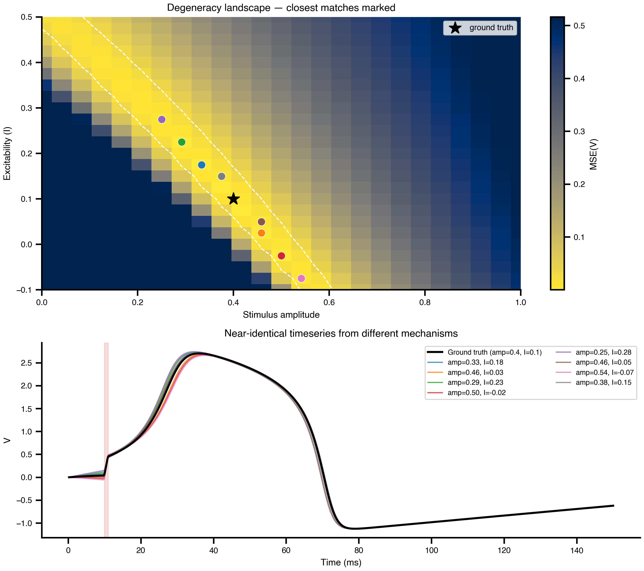
Before any inference, scan the 2D parameter space and compute MSE between the deterministic simulation and the noiseless target at each grid point. The result is the degeneracy landscape: the set of (amplitude, excitability) pairs the data cannot distinguish.
Pick the eight lowest-MSE grid points (excluding a small neighborhood of the ground truth) and overlay their simulated trajectories. They are visually nearly identical despite coming from qualitatively different mechanistic explanations.
Figure 2: The degeneracy ridge. Top: MSE landscape with the eight lowest-loss off-truth grid points marked. Bottom: their simulated trajectories overlaid on the ground truth. They are visually almost identical despite different (amp, I) combinations. This is the ambiguity any inference method has to deal with.
7 Sanity-Checking the Priors
Long MCMC runs hide silent bugs. Before launching one, evaluate the log joint density at two points under scenario C (tight excitability prior). A point with high |I| should score much worse than one with low |I| if the tight prior is actually active. If the two scores come out similar, the priors were dropped during tracing and the whole experiment is wrong.
model_C  log p(amp=0.50, I=0.0):  30.6
model_C  log p(amp=0.10, I=0.3):  -123.3
Difference: 153.8  (should be >> 0 if tight exc prior is active)
8 Running MCMC Under Three Hypotheses
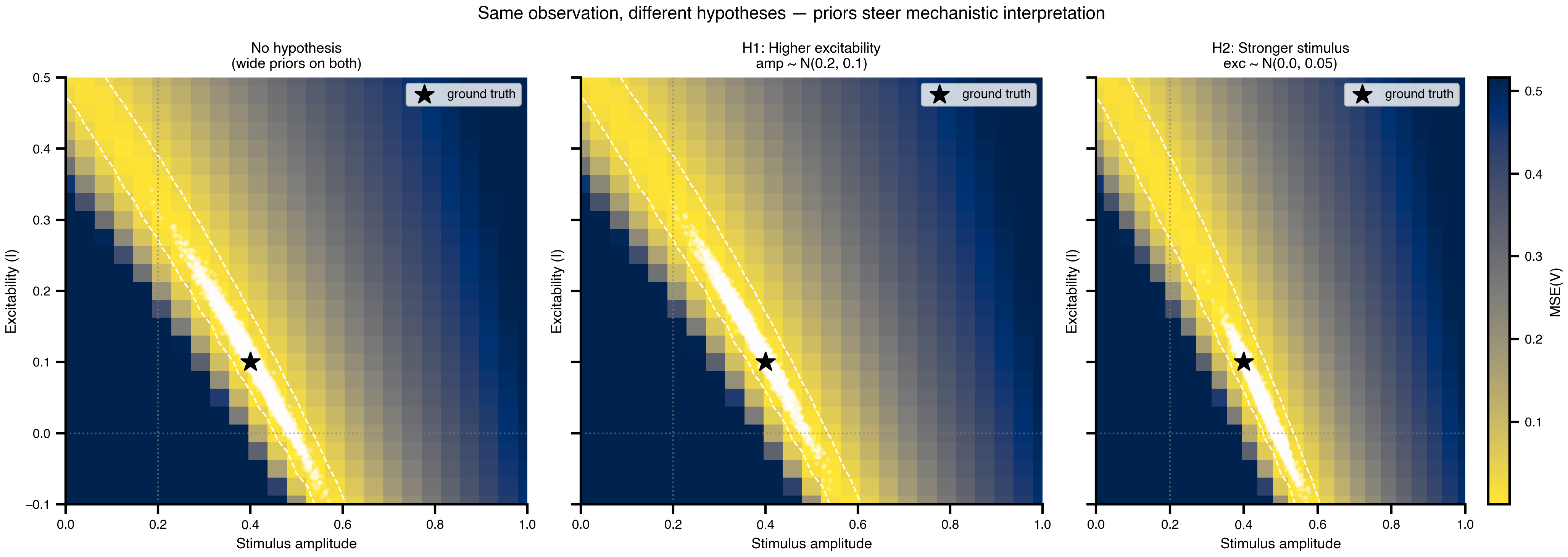
Sample three posteriors with NUTS. dense_mass=True matters here: the posterior is a thin diagonal ridge, and a learned full mass matrix lets the sampler step along the ridge instead of zig-zagging across it.
MCMC_KWARGS =dict(num_warmup=500, num_samples=4000, num_chains=1)# @cache stores the function's return value on disk. On rerun the cached samples# are loaded instead of resampling — set redo=True to force re-running the chain# (e.g. after changing the priors or likelihood).@cache("mcmc_samples", redo=False)def run_all_mcmc():return [ run_mcmc(make_model("A"), seed=0, label="A: No hypothesis (uninformative priors)", **MCMC_KWARGS), run_mcmc(make_model("B"), seed=1, label="H1: Higher excitability (e.g. PET, gene expression)", **MCMC_KWARGS), run_mcmc(make_model("C"), seed=2, label="H2: Stronger stimulus (e.g. device logs, protocol)", **MCMC_KWARGS), ]all_samples = run_all_mcmc()
Figure 3: Joint posteriors overlaid on the degeneracy landscape. Same observation, three hypotheses. Wide priors (A) let samples sprawl along the entire ridge; the tight-amplitude prior (B) confines them to a high-excitability segment; the tight-excitability prior (C) confines them to a high-amplitude segment. The data has not changed across panels, only the slice of the ridge the model is allowed to consider.
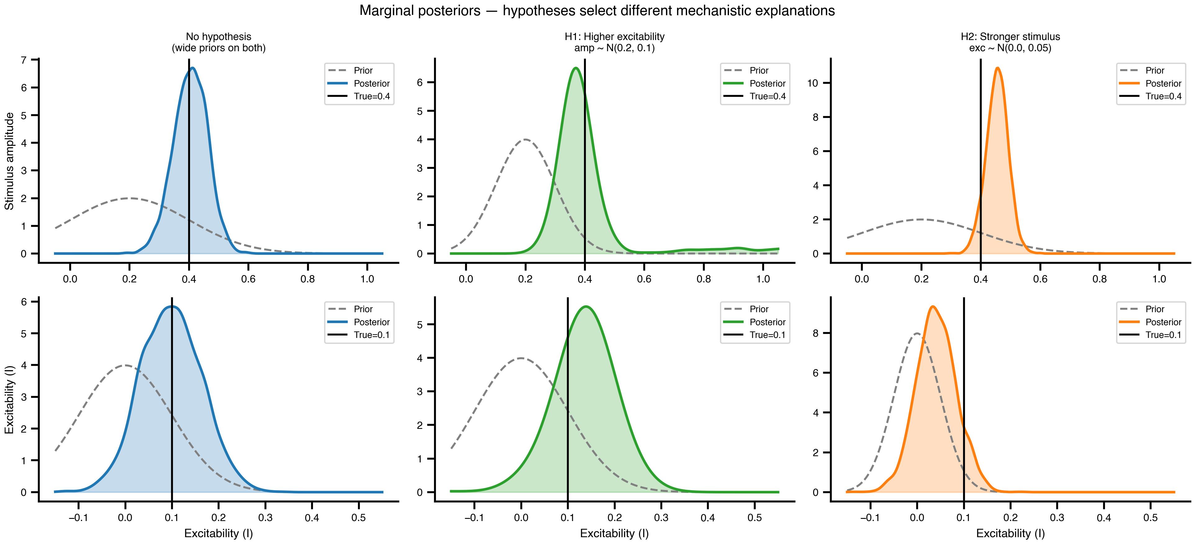
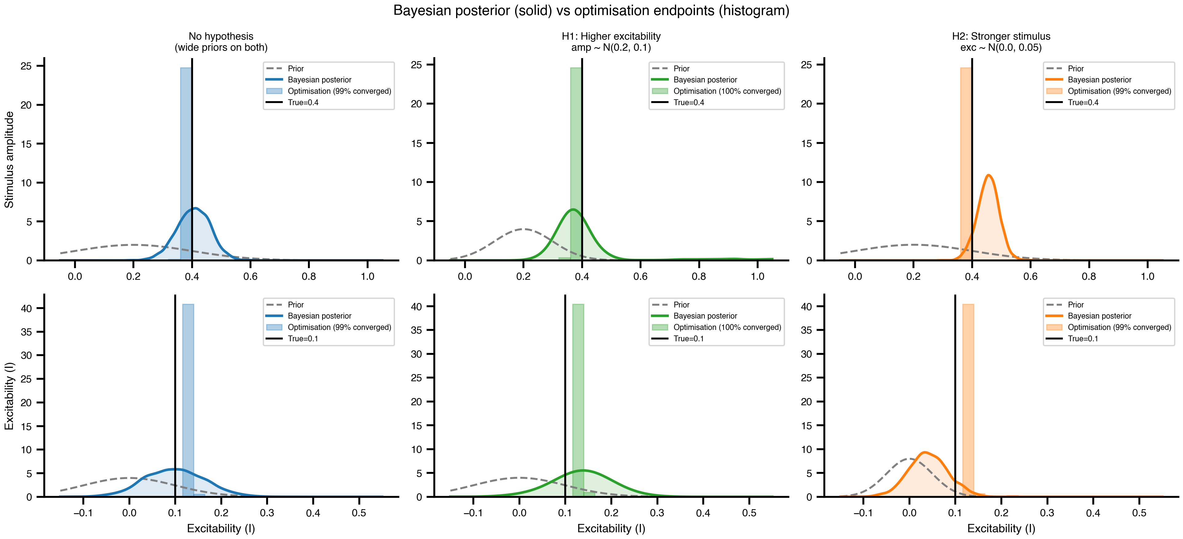
Figure 4: Marginal posteriors versus priors. Dashed grey: prior density. Solid coloured: posterior KDE. Black: ground truth. Top row: amplitude; bottom row: excitability. A wide prior produces a data-driven posterior. A tight prior produces a posterior that tracks the prior, and the other parameter shifts to absorb the discrepancy.
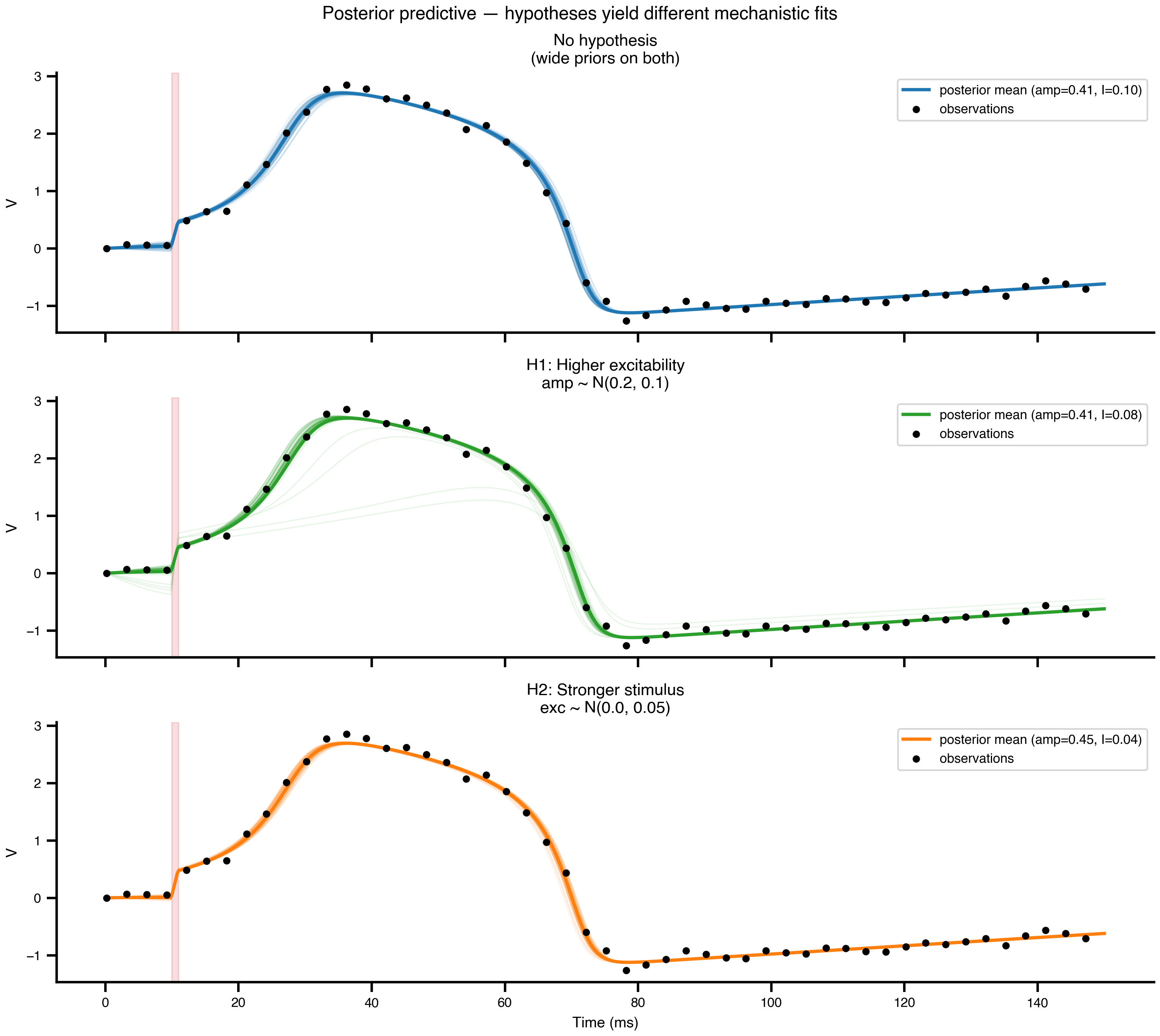
9 Posterior Predictive
Push the posterior back through the forward model: draw N_PP_DRAWS parameter pairs per scenario, simulate each one, overlay the trajectories. The spread of the resulting ensemble is the model’s uncertainty about future observations under that hypothesis, expressed in the same units as the data.
# Semi-transparent traces from posterior draws → uncertainty spread;# posterior-mean prediction as solid line → point summary.N_PP_DRAWS =2* N_DEVICES # must be divisible into N_DEVICES × n_vmappp_traces = {}pp_means = {}for key, samples inzip(SCENARIO_KEYS, all_samples): n_total =len(samples["amplitude"]) draw_idx = jnp.linspace(0, n_total -1, N_PP_DRAWS).astype(int) net_pp = build_network(TRUE_AMPLITUDE, TRUE_EXCITABILITY) sf_pp, cfg_pp = prepare(net_pp, Heun(), t0=0.0, t1=T1, dt=DT) cfg_pp.external.stimulus.amplitude = DataAxis(samples["amplitude"][draw_idx]) cfg_pp.dynamics.I = DataAxis(samples["excitability"][draw_idx]) space_pp = Space(cfg_pp, mode="zip") par_pp = ParallelExecution( model=lambda cfg: sf_pp(cfg).ys[:, 0, 0], space=space_pp, n_pmap=N_DEVICES, n_vmap=N_PP_DRAWS // N_DEVICES, ) results = par_pp.run() pp_traces[key] = jnp.array([results[i] for i inrange(N_PP_DRAWS)]) pp_means[key] = (float(jnp.mean(samples["amplitude"])),float(jnp.mean(samples["excitability"])))print("Posterior predictive simulations complete.")
Figure 5: Posterior-predictive simulations. Faint coloured lines: forward simulations from individual posterior draws. Solid coloured line: simulation at the posterior mean. Black dots: the original observations. All three scenarios fit the data equally well. They disagree only on why.
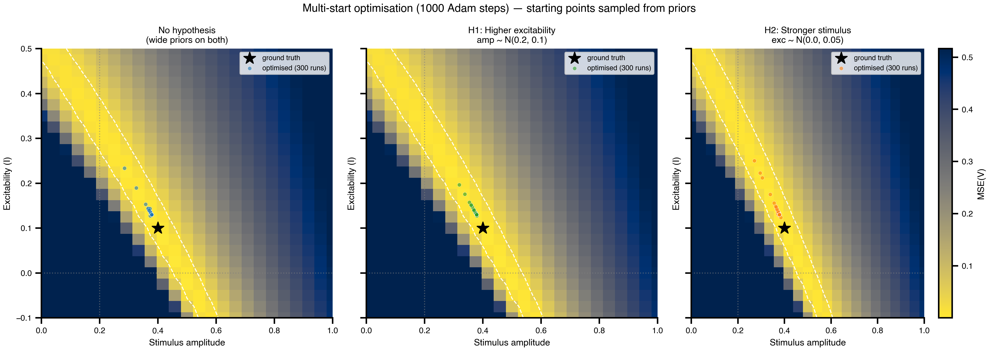
10 Comparison: Multi-Start Optimization
Skip Bayesian inference and run gradient descent instead. Sample starting points from each scenario’s prior, run Adam for 1000 steps from each one. Every run collapses to a single point on the ridge. The optimizer cannot represent the residual uncertainty, and the starting distribution (the prior) decides which segment of the ridge each run lands in.
# Gradient descent from prior-sampled starts reveals:# (a) each run converges to a single point on the ridge — no uncertainty# (b) the starting distribution (prior) determines which ridge segment is found# (c) there is no principled uncertainty quantificationN_SAMPLES =12* N_DEVICESN_OPTIM_STEPS =1000# Cache the multi-start optimisation — 12*N_DEVICES Adam runs per scenario × 3# scenarios is expensive. Set redo=True to rerun after changing learning rate,# step count, or priors.@cache("multistart_optim", redo=False)def run_multistart_optim(): key_opt = jax.random.key(99) opt_results = {}for scenario in SCENARIO_KEYS: key_opt, k_amp, k_exc = jax.random.split(key_opt, 3) amp_starts = PRIOR_AMP_MEAN + PRIOR_AMP_STD[scenario] * jax.random.normal(k_amp, (N_SAMPLES,)) exc_starts = PRIOR_EXC_MEAN + PRIOR_EXC_STD[scenario] * jax.random.normal(k_exc, (N_SAMPLES,)) net_multi = build_network(PRIOR_AMP_MEAN, PRIOR_EXC_MEAN) sf_multi, cfg_multi = prepare(net_multi, Heun(), t0=0.0, t1=T1, dt=DT) cfg_multi.external.stimulus.amplitude = DataAxis(amp_starts) cfg_multi.dynamics.I = DataAxis(exc_starts) space_opt = Space(cfg_multi, mode="zip") optimizer = OptaxOptimizer(make_loss(sf_multi), optax.adam(learning_rate=0.1))def run_optim(config): config.external.stimulus.amplitude = Parameter(config.external.stimulus.amplitude) config.dynamics.I = Parameter(config.dynamics.I) p_fit, _ = optimizer.run(config, max_steps=N_OPTIM_STEPS, chunk_size=N_OPTIM_STEPS)return jnp.array([ collect_parameters(p_fit.external.stimulus.amplitude), collect_parameters(p_fit.dynamics.I), ]) par_opt = ParallelExecution( model=run_optim, space=space_opt, n_pmap=N_DEVICES, n_vmap=N_SAMPLES // N_DEVICES, ) results_opt = par_opt.run() final_params = jnp.array([results_opt[i] for i inrange(N_SAMPLES)]) opt_results[scenario] = {"amplitude": final_params[:, 0],"excitability": final_params[:, 1], }print(f"Scenario {scenario}: {N_SAMPLES} optimisations complete.")return opt_resultsopt_results = run_multistart_optim()
Figure 6: Multi-start optimization endpoints. Each coloured dot is the final (amp, I) of one gradient-descent run. Endpoints cluster onto narrow regions of the ridge, but those regions just track where the starting points (sampled from the prior) happened to lie. The clustering is not a posterior. It is a smeared-out projection of the prior, with no notion of uncertainty attached.
Figure 7: Bayesian posteriors vs optimization endpoints, side by side. Solid lines: Bayesian posterior densities. Translucent histograms: optimization endpoints from the same priors. The two are answers to different questions. Optimization tells you where the loss is low given a starting bias. Bayes tells you what to believe about the parameter given the data and a prior.
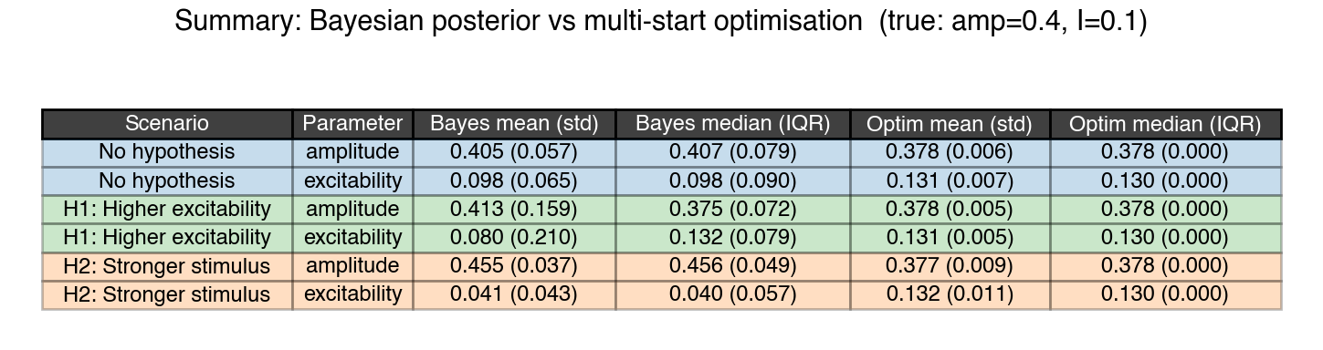
11 Summary Table
The per-scenario numbers in one place. For each parameter and each scenario: mean and std, median and IQR, computed once from the Bayesian posterior and once from the multi-start optimization endpoints.
Figure 8: Summary statistics by scenario and method. For each scenario (A/B/C) and each parameter (amplitude, excitability), we report mean ± std and median ± IQR for the Bayesian posterior and for the multi-start optimization endpoints. Compare across rows to see how the same observation produces different inferences under different hypotheses.
Takeaways
The forward model is degenerate: a ridge of (amplitude, excitability) pairs produces near-identical observations.
Optimization collapses that ridge to a single arbitrary point. It is silent about residual uncertainty.
Bayesian inference returns the full posterior along the ridge. The prior is where mechanistic evidence (a PET scan, a stimulator log) enters in a way the optimizer cannot represent.
All three scenarios fit the data equally well. They differ only in which mechanistic explanation they prefer. That is the practical payoff of making priors explicit.
12 Exercises & Exploration
Shrink LIKELIHOOD_SIGMA by an order of magnitude. Does the posterior tighten around the truth, or does the ridge persist?
Change the pulse ONSET or DURATION and regenerate the observation. How do the three posteriors react to a different stimulation protocol?
Set dense_mass=False on the NUTS sampler. Inspect the effective sample size. How much worse does the sampler do on the ridge geometry?
Reduce the observation density: change obs_idx = jnp.arange(0, len(ts), 15) to jnp.arange(0, len(ts), 30). Half as many observations — how much wider does the posterior get?
Swap optax.adam for optax.adamaxw in the multi-start optimisation. The endpoints spread along the ridge instead of collapsing onto a single point. Why does the choice of optimiser change which segment of the ridge gets covered?