Goal

Authors

Affiliations

Marius Pille

Berlin Institute of Health at Charité University Medicine

Leon Martin

Berlin Institute of Health at Charité University Medicine

Leon Stefanovski

Charité University Medicine Berlin

Use a TVB-O SimulationExperiment with a stimulus defined as an Event. Compare the resting and stimulated time series.

from tvbo import Dynamics, SimulationExperiment
from tvbo.datamodel.schema import Event

1 1. A baseline experiment

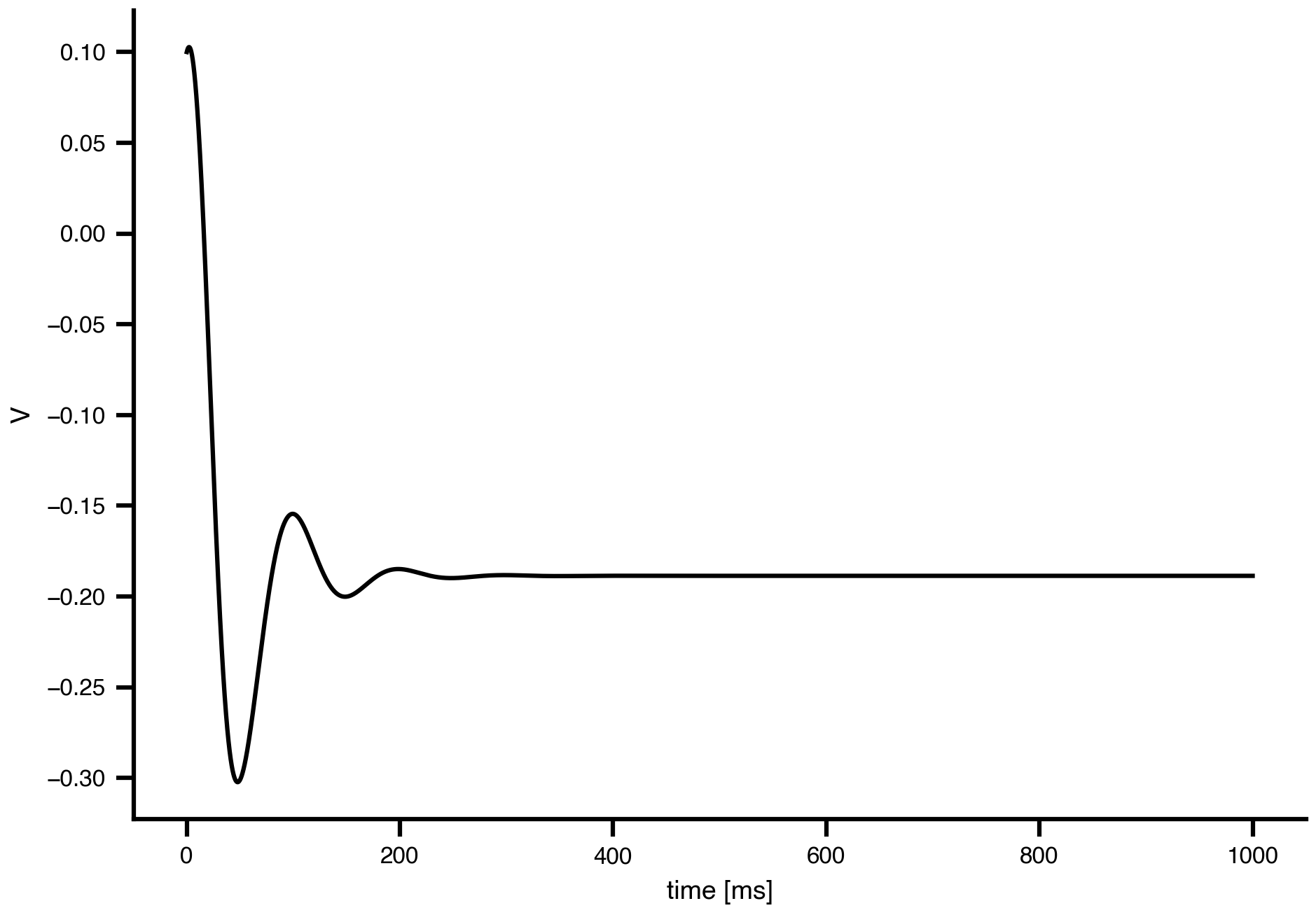
Start with the Generic2dOscillator (G2D) and its database defaults. The trajectory relaxes onto a stable focus at V ≈ −0.19. These parameters are far from any oscillation.

g2d = Dynamics.from_db("Generic2dOscillator")

exp = SimulationExperiment(dynamics=g2d)
res = exp.run()
res.integration.sel(variable="V").plot()


============================================================
STEP 1: Running simulation...
============================================================
  Simulation period: 1000.0 ms, dt: 0.01220703125 ms
  Transient period: 0.0 ms
  Simulation complete.

============================================================
Experiment complete.
============================================================

2 2. Define a stimulus as an `Event`

An Event is a symbolic, time-dependent perturbation. Here, a rectangular pulse is defined using Piecewise. Any expression in t and the event’s parameters is valid.

event = Event(
    name="perturbation",
    event_type="stimulus",
    parameters={
        "onset":     {"value": 200.0},
        "width":     {"value": 200.0},
        "amplitude": {"value": 1.0},
    },
    equation={
        "rhs": "Piecewise((amplitude, (t >= onset) & (t < onset + width)), (0.0, True))"
    },
)
event.plot();

Note

The default G2D enters the oscillatory regime at I ≈ 3.7 (lower Hopf). At I + perturbation = 5, the system is above the Hopf, so a limit cycle appears during the pulse.

3 3. Inject the event into the model

Steps: 1. Register the event under exp.events["<name>"]. 2. Edit the right-hand side of the state variable to be driven. Here, for V, replace the constant input I with (I + perturbation).

exp.events["perturbation"] = event
exp.dynamics.state_variables["V"].equation.rhs = (
    "d*tau*((I + perturbation)*gamma - V**3*f + V**2*e + V*g "
    "+ V*local_coupling + W*alpha + c_glob*gamma)"
)

Widen the W domain before running

G2D uses W ∈ [−6, 6] as its state-variable domain. The JAX kernel wraps Heun in a BoundedSolver that clamps W at those limits. At I = 5, the limit cycle swings W down to about −9, so the solver pins W at −6. V then settles on the cubic’s right branch at V ≈ 2.88, a square plateau rather than an oscillation. Widen the domain before running.

import matplotlib.pyplot as plt
fig, ax = plt.subplots()
exp.dynamics.state_variables["W"].domain.lo = -20.0
exp.dynamics.state_variables["W"].domain.hi = 20.0

res_stim = exp.run()
res_stim.integration.sel(variable="V").plot(ax=ax)
ax2=ax.twinx()
event.plot(ax=ax2, alpha=0.5, linestyle=':')


============================================================
STEP 1: Running simulation...
============================================================
  Simulation period: 1000.0 ms, dt: 0.01220703125 ms
  Transient period: 0.0 ms
  Simulation complete.

============================================================
Experiment complete.
============================================================

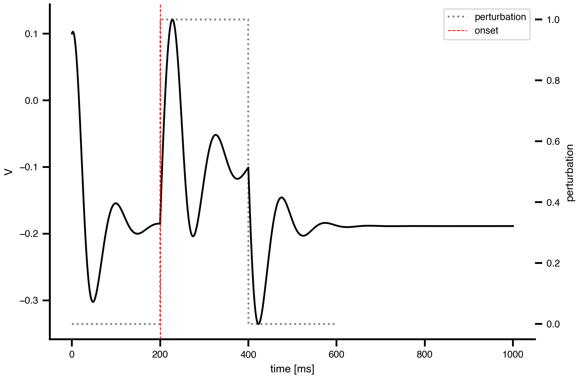
Now the trajectory oscillates during the pulse and returns to the stable focus after.

4 4. Five-node motif: stimulus propagation

The five-region motif below uses the same parameter regime as the Bayesian workshop example. The stimulus is brief, so R0 gives one evoked response rather than a long driven oscillation. Edge weights and tract lengths live in edge parameters, and network.plot_overview() shows the directed motif.

R0 is the stimulated site (peripheral). The stimulus reaches R1 through a short 30 mm branch and R3 through a longer 100 mm branch. R1 and R3 are hyperexcitable branch nodes. R2 and R4 are quiet leaves.

Coupling gain

Use a = 0.1, matching the workshop example. The node excitabilities are I = [0.05, 0.30, 0.05, 0.25, 0.05]: R1 and R3 are hot, R0, R2, and R4 are quiet.

from tvbo import Network, SimulationExperiment, Dynamics, Coupling
from tvbo.datamodel.schema import Event

T1 = 150.0
DT = 0.2
ONSET = 10.0
DURATION = 1.0
G_COUPLING = 0.1
TRUE_AMPLITUDE = 0.4
DYNAMICS_PARAMS = {
    "a": -1.5,
    "b": -15.0,
    "c": 0.0,
    "d": 0.015,
    "e": 3.0,
    "f": 1.0,
    "tau": 4.0,
}

network_yaml = """
label: StimPropagationMotif
number_of_nodes: 5
nodes:
    - {id: 0, label: R0, description: "stimulated site, peripheral, quiet", parameters: {I: {value: 0.05}}}
    - {id: 1, label: R1, description: "hub, hyperexcitable", parameters: {I: {value: 0.30}}}
    - {id: 2, label: R2, description: "quiet leaf", parameters: {I: {value: 0.05}}}
    - {id: 3, label: R3, description: "hyperexcitable branch node", parameters: {I: {value: 0.25}}}
    - {id: 4, label: R4, description: "quiet leaf", parameters: {I: {value: 0.05}}}
edges:
    - {source: 0, target: 1, directed: true, parameters: {weight: {value: .1}, length: {value: 30.0, unit: mm}}}
    - {source: 0, target: 3, directed: true, parameters: {weight: {value: .1}, length: {value: 100.0, unit: mm}}}
    - {source: 3, target: 4, directed: true, parameters: {weight: {value: .1}, length: {value: 30.0, unit: mm}}}
    - {source: 1, target: 2, directed: true, parameters: {weight: {value: .1}, length: {value: 30.0, unit: mm}}}
"""

network = Network.from_string(network_yaml)

network.plot_overview()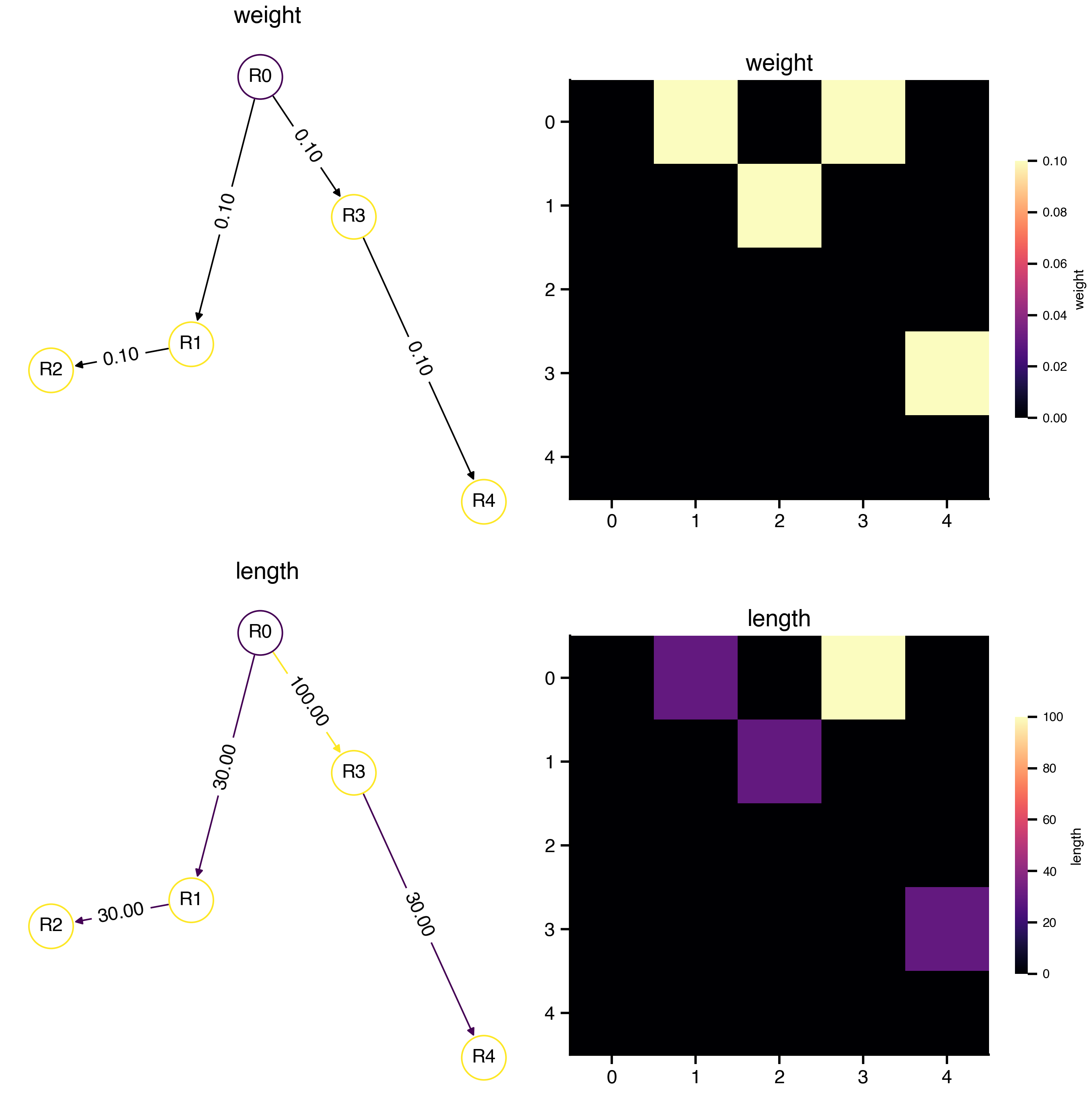

event = Event(
    name="perturbation",
    event_type="stimulus",
    parameters={
        "onset": {"value": ONSET},
        "duration": {"value": DURATION},
        "amplitude": {"value": TRUE_AMPLITUDE},
    },
    equation={"rhs": "Piecewise((amplitude, (t >= onset) & (t < onset + duration)), (0.0, True))"},
    regions=[0],
    weighting=[1.0],
)

dynamics = Dynamics.from_db("Generic2dOscillator")
for name, value in DYNAMICS_PARAMS.items():
    dynamics.parameters[name].value = value

exp = SimulationExperiment(
    dynamics=dynamics,
    coupling=Coupling(name="Linear", parameters={"a": {"value": G_COUPLING}, "b": {"value": 0.0}}),
    network=network,
)
exp.events["perturbation"] = event

exp.dynamics.state_variables["V"].equation.rhs = (
    "d*tau*((I + perturbation)*gamma - V**3*f + V**2*e + V*g "
    "+ V*local_coupling + W*alpha + c_glob*gamma)"
)
exp.integration.duration = T1
exp.integration.step_size = DT

res = exp.run()


============================================================
STEP 1: Running simulation...
============================================================
  Simulation period: 150.0 ms, dt: 0.2 ms
  Transient period: 0.0 ms
  Simulation complete.

============================================================
Experiment complete.
============================================================

fig, ax = plt.subplots()
res.integration.sel(variable="V").plot(ax=ax)
ax2 = ax.twinx()
event.plot(ax=ax2, color="grey")
leg = ax2.get_legend()
leg.set_loc('lower right')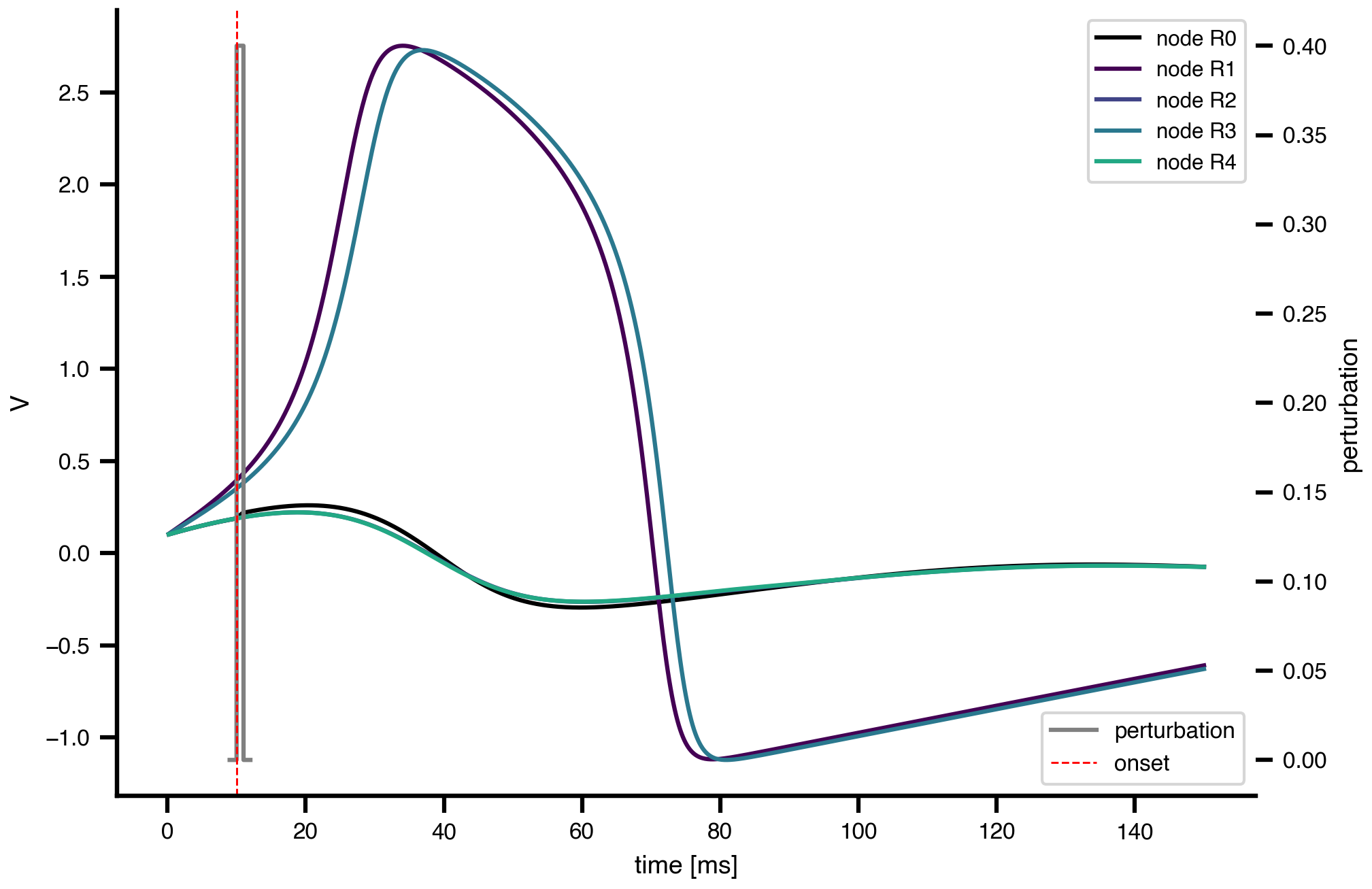

Run the same experiment again with a slower transmission speed. The edge lengths are unchanged; only conduction_speed changes, so delays scale as length / conduction_speed.

SLOW_CONDUCTION_SPEED = 1

slow_network = Network.from_string(network_yaml)
slow_network.parameters["conduction_speed"].value = SLOW_CONDUCTION_SPEED

slow_dynamics = Dynamics.from_db("Generic2dOscillator")
for name, value in DYNAMICS_PARAMS.items():
    slow_dynamics.parameters[name].value = value

slow_exp = SimulationExperiment(
    dynamics=slow_dynamics,
    coupling=Coupling(name="Linear", parameters={"a": {"value": G_COUPLING}, "b": {"value": 0.0}}),
    network=slow_network,
)
slow_exp.events["perturbation"] = event
slow_exp.dynamics.state_variables["V"].equation.rhs = exp.dynamics.state_variables["V"].equation.rhs
slow_exp.integration.duration = T1
slow_exp.integration.step_size = DT

slow_res = slow_exp.run()

fig, ax = plt.subplots()
slow_res.integration.sel(variable="V").plot(ax=ax)
ax2 = ax.twinx()
event.plot(ax=ax2, color="grey")
leg = ax2.get_legend()
leg.set_loc("lower right")


============================================================
STEP 1: Running simulation...
============================================================
  Simulation period: 150.0 ms, dt: 0.2 ms
  Transient period: 0.0 ms
  Simulation complete.

============================================================
Experiment complete.
============================================================

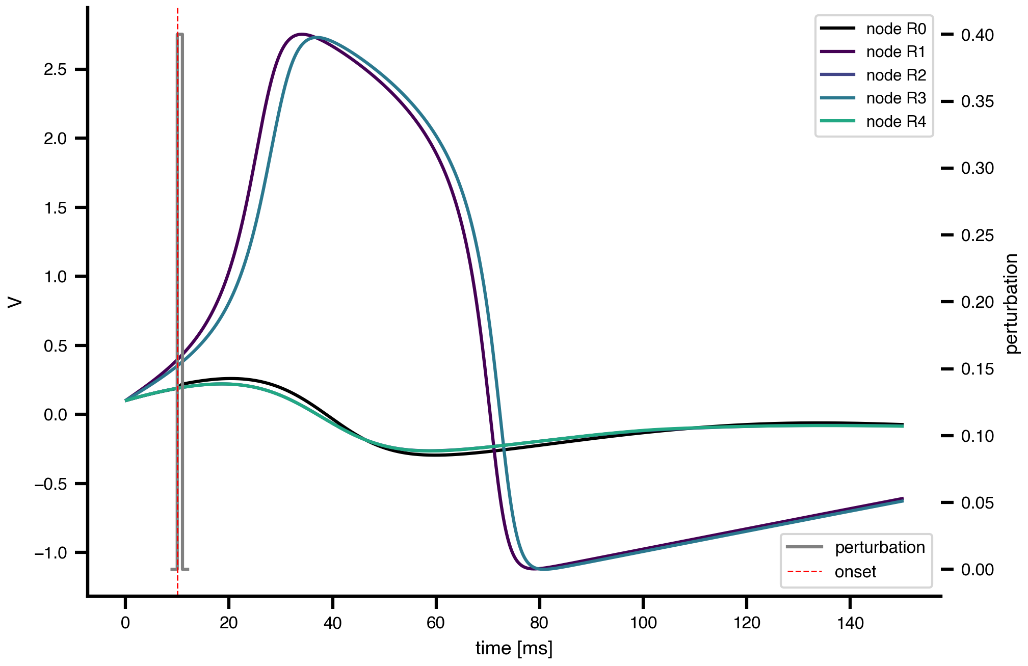
Result: The current pulse starts at 10 ms and lasts 1 ms. Compare the two plots: slowing conduction speed stretches propagation along the direct branches from R0, so the longer R0-to-R3 branch lags more clearly behind the shorter R0-to-R1 branch.

5 Exercises

Iso-energy comparison. Keep the energy amplitude × width constant but shrink width (e.g. width=20, amplitude=50 instead of width=200, amplitude=5). Plot the response. Is a brief, strong kick more or less efficient at triggering the limit cycle than a long, gentle one? Consider the system’s relaxation time vs. the pulse duration.
Phase / timing effects. Once the system is on the limit cycle, the response to a second pulse depends on when it arrives within the cycle. Re-run with two events (exp.events["pulse1"], exp.events["pulse2"]) at the same amplitude but different onset values offset by a fraction of the cycle period. Compare the trajectories and look for constructive or destructive interference.
Sub-threshold pulse. Reduce amplitude to 0.1 and re-run. You should see only a small damped twitch around the pulse, because the system never leaves the basin of the stable fixed point.
Closer to the bifurcation. Set the baseline I (exp.dynamics.parameters["I"].value = 2.9) and re-run with a small amplitude. A tiny perturbation now triggers oscillations.
Different waveform. Replace the Piecewise rhs with a Gaussian, amplitude*exp(-((t-onset)/width)**2), and observe the smoother response.
Different target. Inject the event into W instead of V by editing exp.dynamics.state_variables["W"].equation.rhs.

1 1. A baseline experiment

2 2. Define a stimulus as an Event

3 3. Inject the event into the model

4 4. Five-node motif: stimulus propagation

5 Exercises

2 2. Define a stimulus as an `Event`