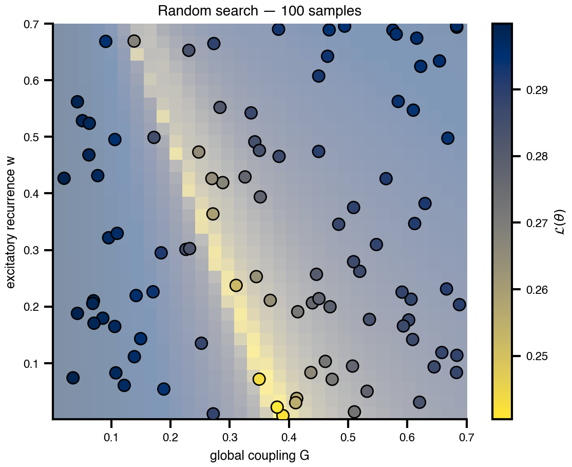
Bergstra, James, and Yoshua Bengio. 2012.
“Random Search for Hyper-Parameter Optimization.” Journal of Machine Learning Research 13 (null): 281–305.
https://dl.acm.org/doi/abs/10.5555/2188385.2188395.
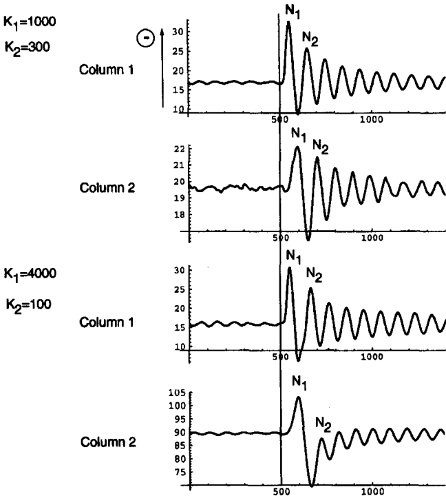
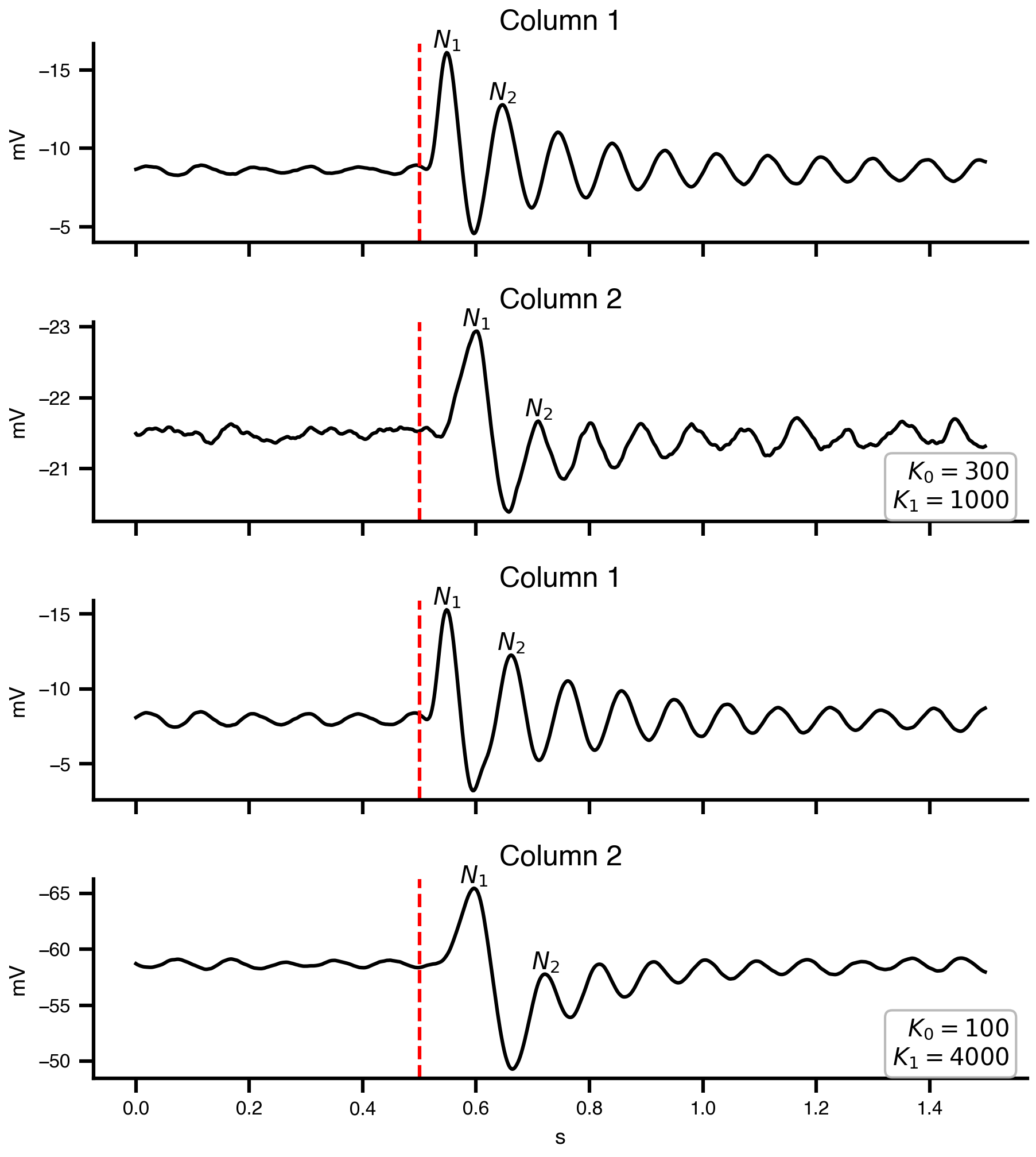
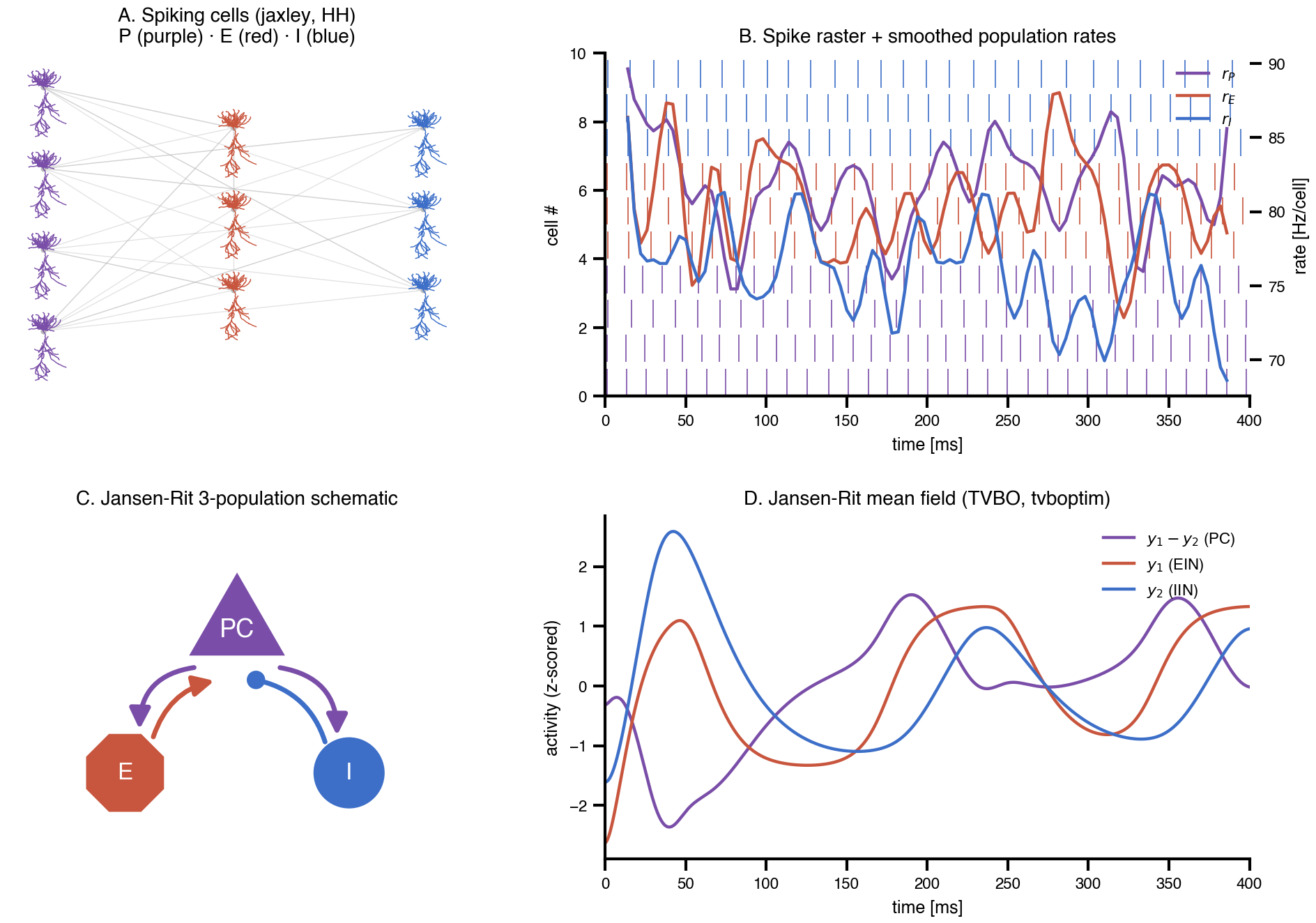
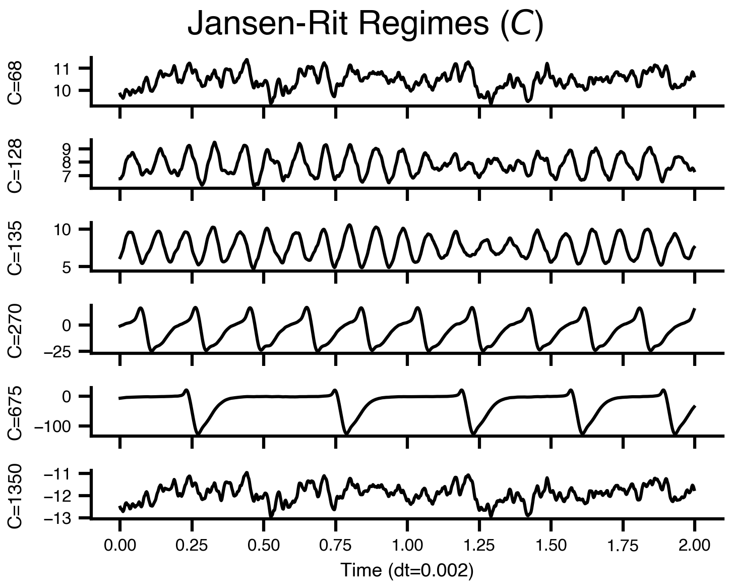
Jansen, Ben H., and Vincent G. Rit. 1995.
“Electroencephalogram and Visual Evoked Potential Generation in a Mathematical Model of Coupled Cortical Columns.” Biological Cybernetics 73 (4): 357–66.
https://doi.org/10.1007/bf00199471.
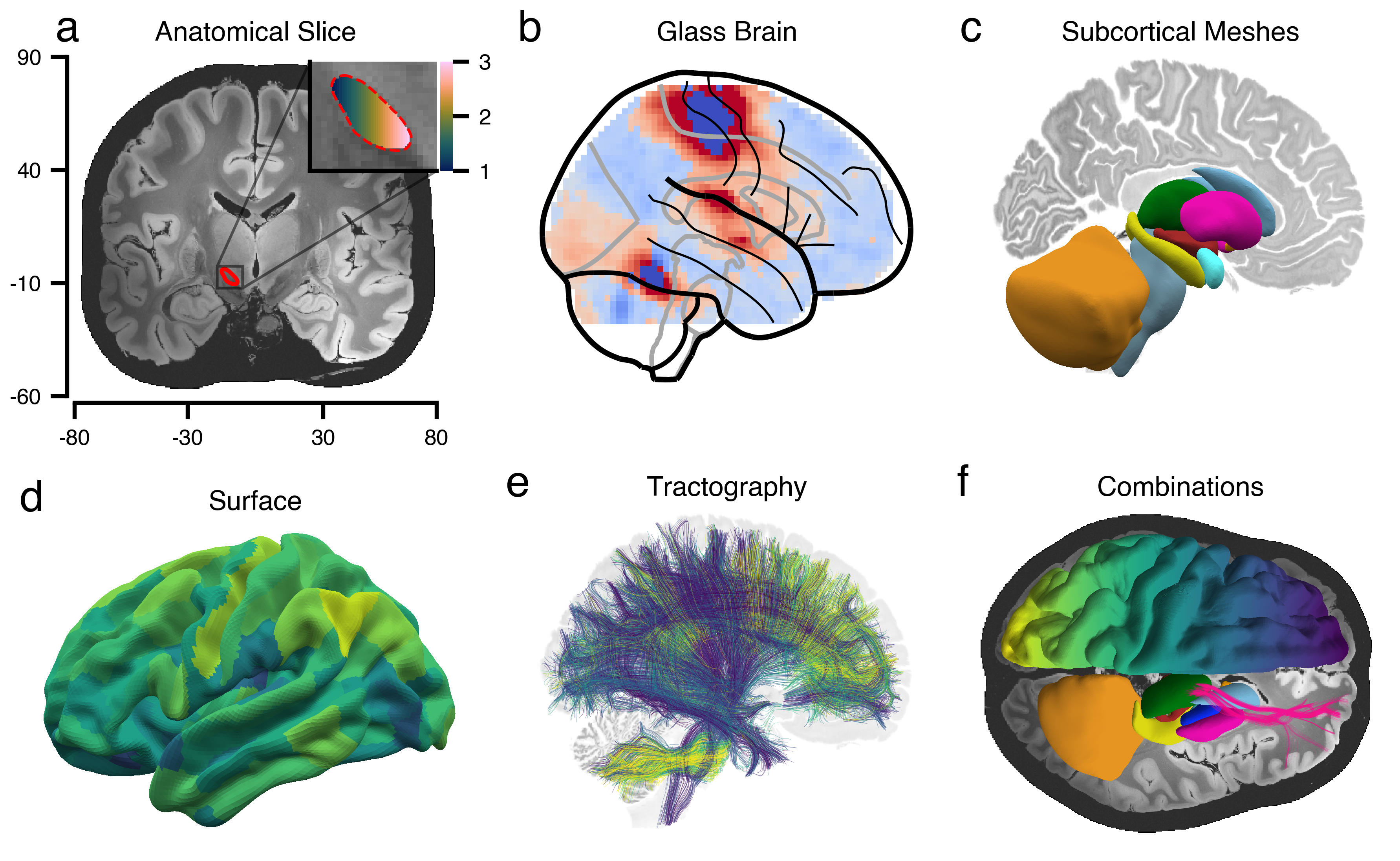
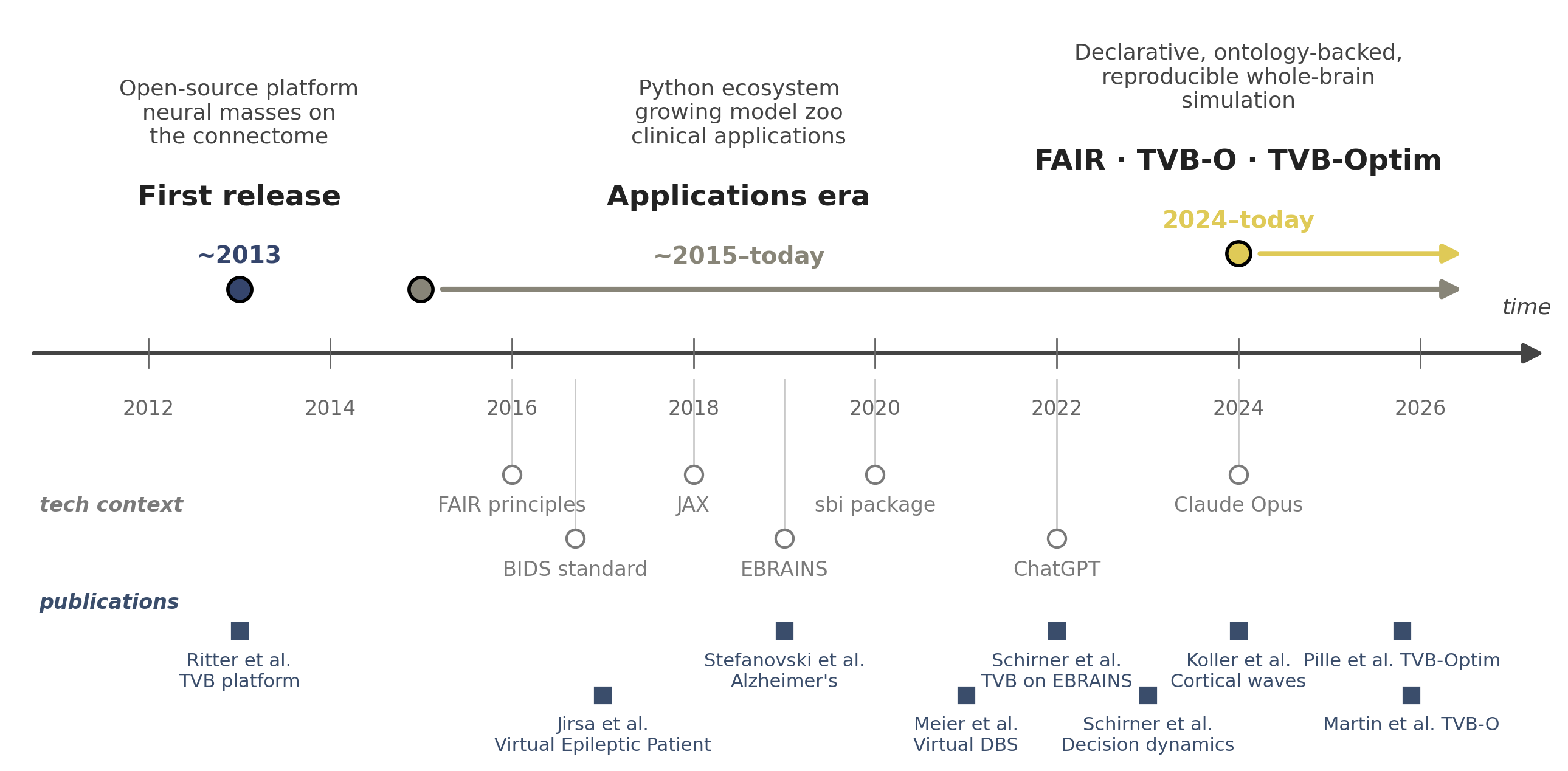
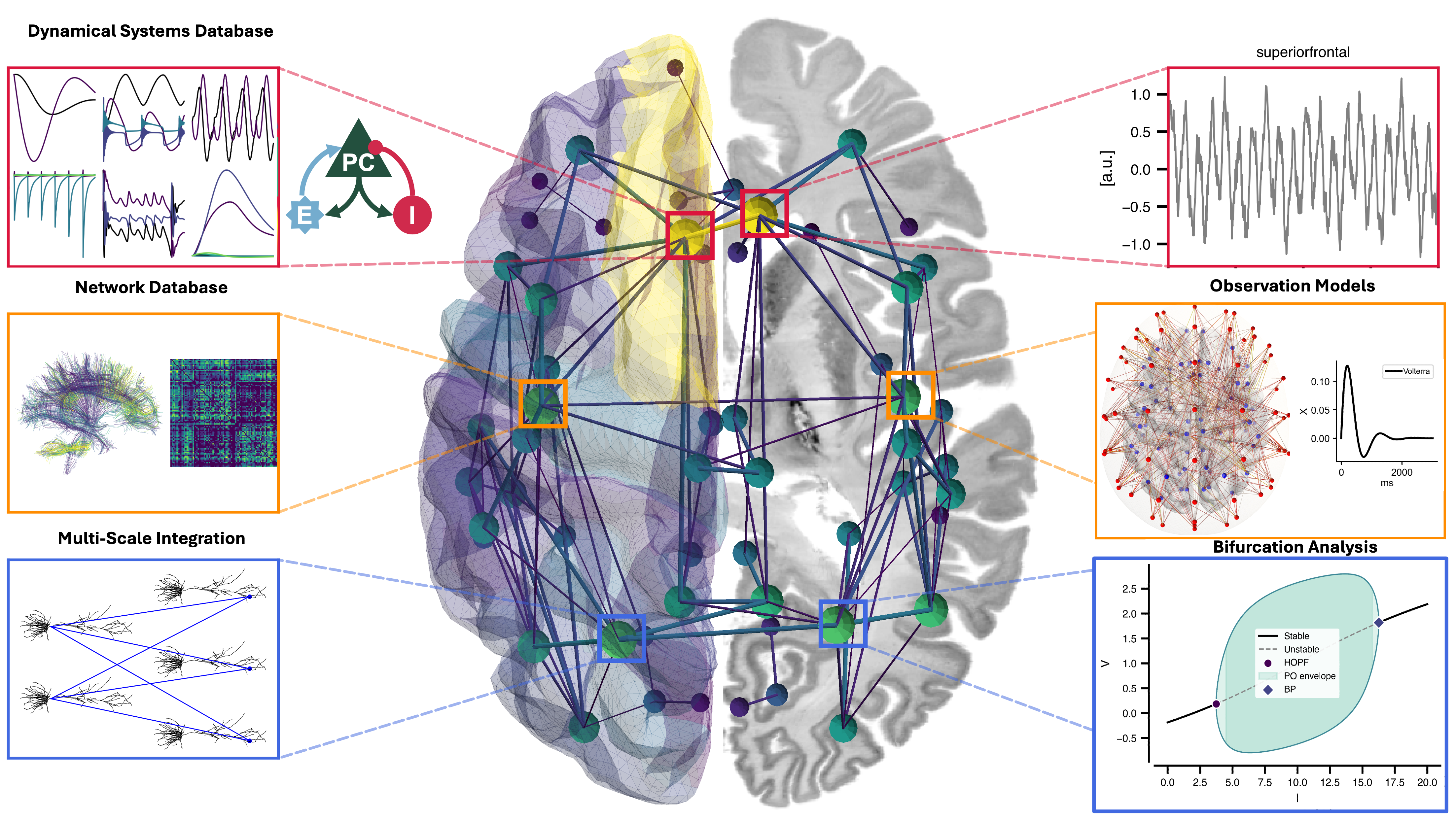
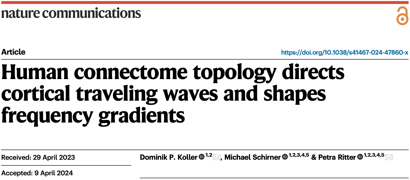
Koller, Dominik P., Michael Schirner, and Petra Ritter. 2024.
“Human Connectome Topology Directs Cortical Traveling Waves and Shapes Frequency Gradients.” Nature Communications 15 (1).
https://doi.org/10.1038/s41467-024-47860-x.
Kuramoto, Yoshiki. 1975.
“Self-Entrainment of a Population of Coupled Non-Linear Oscillators.” In
Lecture Notes in Physics, 420–22. Springer-Verlag.
https://doi.org/10.1007/bfb0013365.
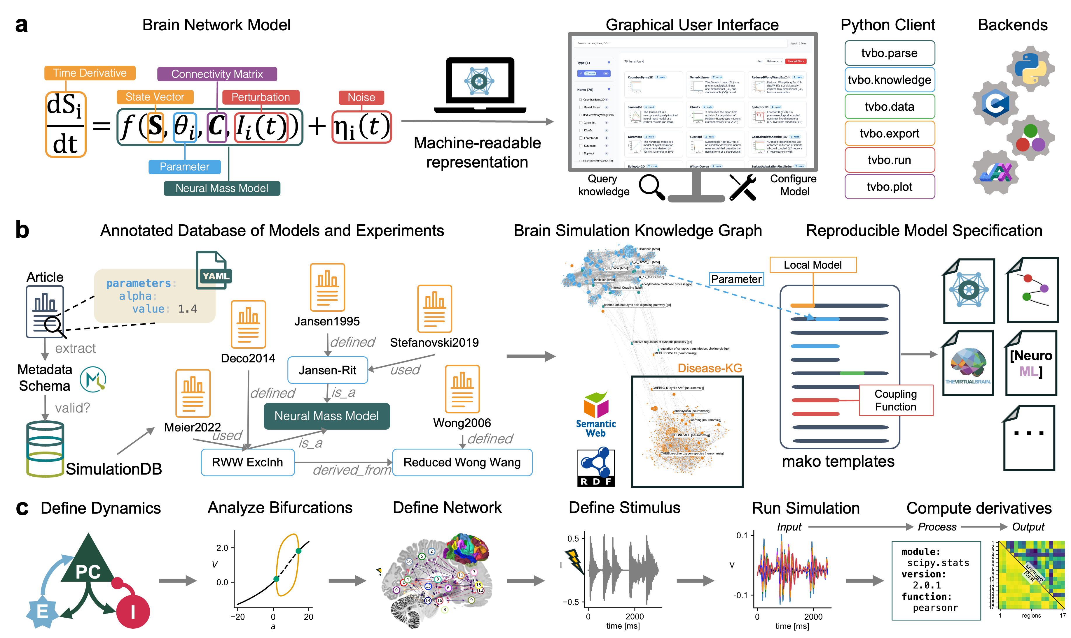
Martin, Leon, Konstantin Buelau, Marius Pille, Rico Andre Schmitt, Christoph Huettl, Jil M Meier, Halgurd Taher, Dionysios Perdikis, Michael Schirner, and Petra Ritter. 2025.
“The Virtual Brain Ontology: A Digital Knowledge Framework for Reproducible Brain Network Modeling.” bioRxiv, November.
https://doi.org/10.1101/2025.11.19.689211.
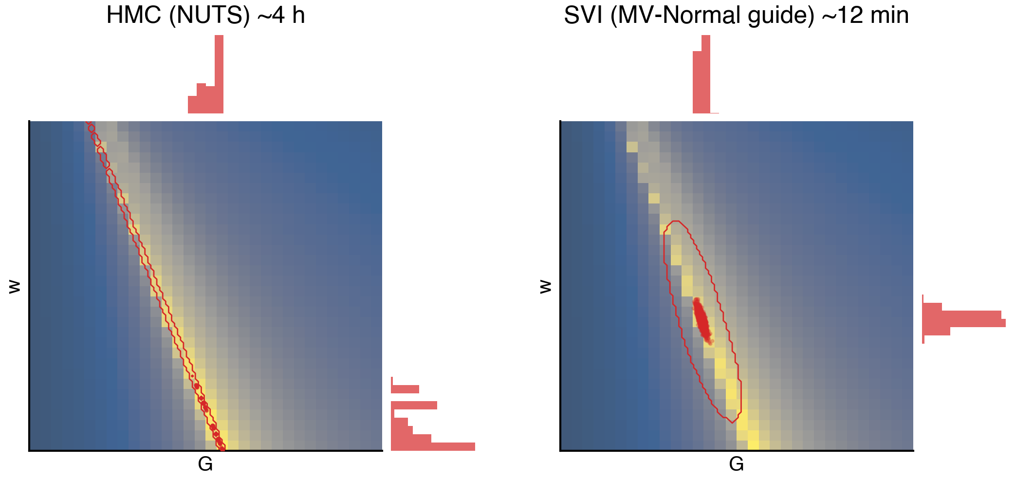
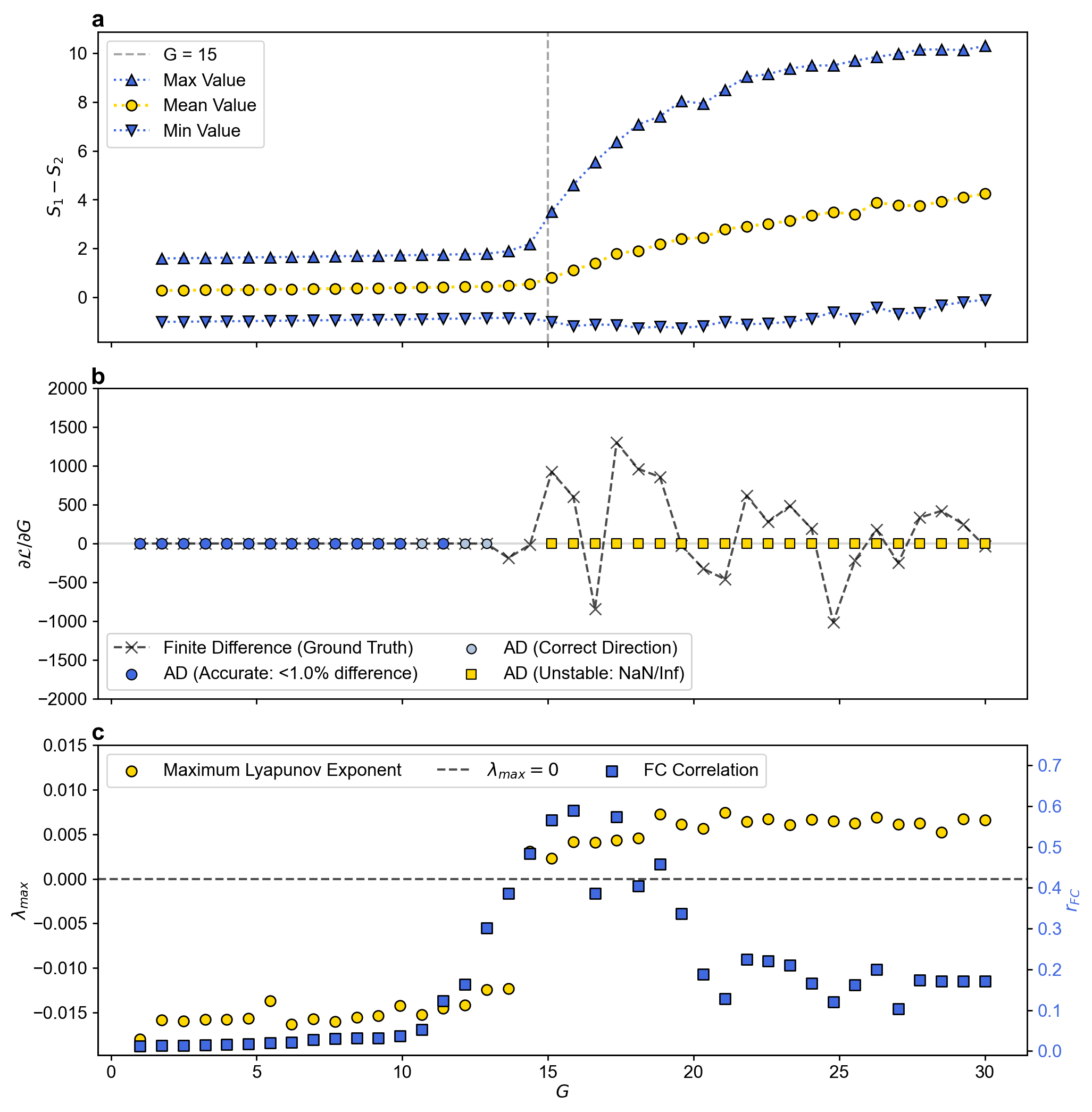
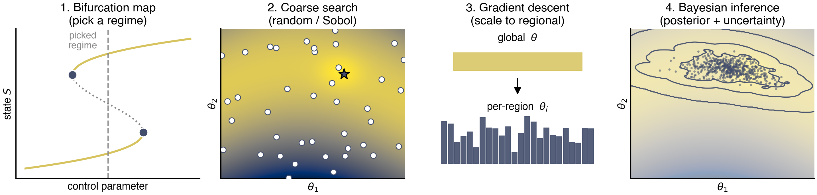
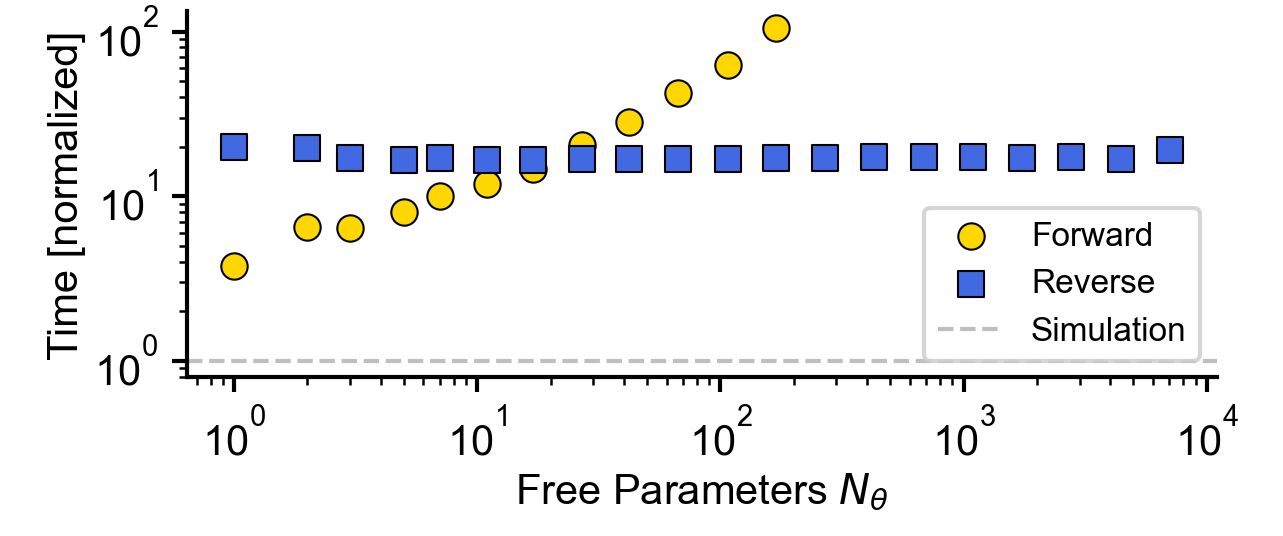
Pille, Marius, Leon Martin, Emilius Richter, Dionysios Perdikis, Michael Schirner, and Petra Ritter. 2025.
“Fast and Easy Whole-Brain Network Model Parameter Estimation with Automatic Differentiation.” bioRxiv, November.
https://doi.org/10.1101/2025.11.18.689003.
Schirner, Michael, Gustavo Deco, and Petra Ritter. 2023.
“Learning How Network Structure Shapes Decision-Making for Bio-Inspired Computing.” Nature Communications 14 (1).
https://doi.org/10.1038/s41467-023-38626-y.


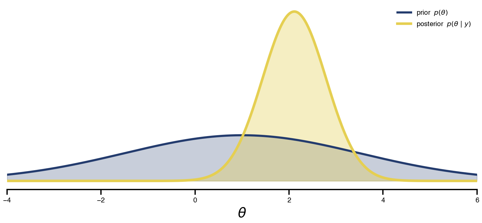
 Flat / uninformative:
  Weakly informative:
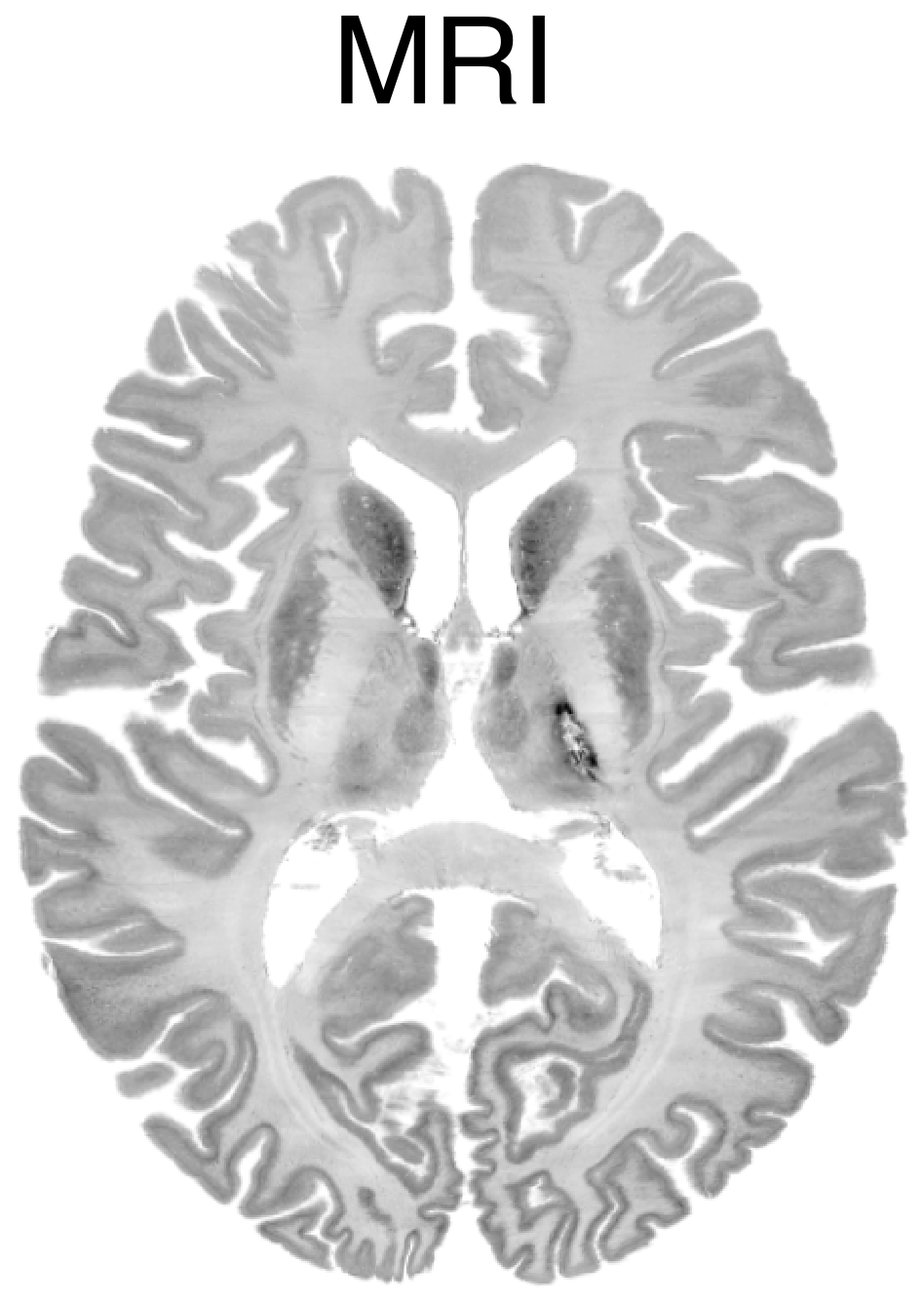
  Strongly informative: derived from independent measurements: anatomy, tau / amyloid PET maps, receptor density, EEG power. “This patient’s region has elevated tau” → prior on local excitation per region.