Dynamical Systems with TVBO: A Spring-Mass Example

Authors

Affiliations

Marius Pille

Berlin Institute of Health at Charité University Medicine

Leon Martin

Berlin Institute of Health at Charité University Medicine

Leon Stefanovski

Charité University Medicine Berlin

import bsplot
import matplotlib.pyplot as plt
import numpy as np
from IPython.display import Markdown

from tvbo import Dynamics, SimulationExperiment
from tvbo.datamodel.schema import Exploration, ExplorationAxis

bsplot.style.use("tvbo")

1 Dynamical Systems

This notebook is the static companion to the workshop slides. The slides show the same concepts visually; here we make them explicit in TVBO code.

The workshop starts from the generic state-evolution equation

\[ dS_i = \left[f_d(S_i, \theta^d, C_i, I_i)\right]dt + g(S_i, \theta^g)\,dW_i. \]

Here we remove everything except deterministic local dynamics: one system, no coupling, no external input, and no noise. That leaves the core object that appears throughout TVBO: a dynamical system with state variables, parameters, initial conditions, and equations of motion.

\[ dS_i = f(S_i, \theta) \]

1.1 Learning Path

1. Specify a dynamical system as a TVBO Dynamics object.
2. Put it in a SimulationExperiment and run it with tvboptim.
3. Read results through named dimensions.
4. Compare initial conditions as trajectories in the same flow.
5. Use phase space to see the geometry of the dynamics.
6. Vary parameters declaratively with Exploration.
7. Add damping and load terms to move from a toy model toward realism.

1.2 From a Second-Order Equation to TVBO

A mass \(m\) attached to a spring with stiffness \(k\) satisfies

\[ m\ddot{x} = -kx. \]

Numerical ODE solvers work with first-order systems, so we introduce velocity \(v = \dot{x}\):

\[ \dot{x} = v, \qquad \dot{v} = -\frac{k}{m}x. \]

In TVBO, we write this directly as metadata: state variables, equations, parameters, units, and initial values.

spring = Dynamics(
    name="SpringMass",
    description="Undamped spring-mass oscillator in first-order form.",
    state_variables={
        "x": {
            "description": "Displacement from equilibrium",
            "unit": "m",
            "equation": {"rhs": "v"},
            "initial_value": 2.0,
        },
        "v": {
            "description": "Velocity",
            "unit": "m_per_s",
            "equation": {"rhs": "-(k/m) * x"},
            "initial_value": 0.0,
        },
    },
    parameters={
        "k": {
            "description": "Spring stiffness",
            "unit": "N_per_m",
            "value": 0.0001,
        },
        "m": {
            "description": "Mass",
            "unit": "kg",
            "value": 1.0,
        },
    },
)

print(spring.render('yaml'))

name: SpringMass
parameters:
  k:
    name: k
    value: 0.0001
    description: Spring stiffness
    unit: N_per_m
  m:
    name: m
    value: 1.0
    description: Mass
    unit: kg
description: Undamped spring-mass oscillator in first-order form.
state_variables:
  x:
    name: x
    description: Displacement from equilibrium
    equation:
      lhs: Derivative(x, t)
      rhs: v
      latex: false
    unit: m
    record: true
    variable_of_interest: true
    coupling_variable: false
    equation_type: differential
    equation_order: 1
    initial_value: 2.0
  v:
    name: v
    description: Velocity
    equation:
      lhs: Derivative(v, t)
      rhs: -k*x/m
      latex: false
    unit: m_per_s
    record: true
    variable_of_interest: true
    coupling_variable: false
    equation_type: differential
    equation_order: 1
    initial_value: 0.0
number_of_modes: 1
autonomous: true

Each TVB-O element can also render a Markdown report. This enables the user to double-check the equations and specification in human-readable format.

Markdown(spring.render("markdown"))

SpringMass

Undamped spring-mass oscillator in first-order form.

autonomous: True; modes: 1; state variables: 2; parameters: 2.

State Equations

\[ \dot{x} = v \] \[ \dot{v} = - \frac{k*x}{m} \]

State Variables

Variable	Initial Value	Unit	Equation	Domain / Sampling	Flags	Description
\(x\)	2.0	\(\mathrm{m}\)	differential (order 1)	—	VOI, recorded	Displacement from equilibrium
\(v\)	0.0	\(\frac{\mathrm{m}}{\mathrm{s}}\)	differential (order 1)	—	VOI, recorded	Velocity

Parameters

Parameter	Value	Default	Unit	Domain / Sampling	Flags	Description
\(k\)	0.0001	—	\(\frac{\mathrm{N}}{\mathrm{m}}\)	—	—	Spring stiffness
\(m\)	1.0	—	\(\mathrm{kg}\)	—	—	Mass

1.3 Run a Simulation Experiment

For the workshop workflow we usually wrap the model in a SimulationExperiment. The model still describes the equations; the experiment describes how to run them. The SimulationExperiment contains all metadata relevant to run it with different software backends.

experiment = SimulationExperiment(dynamics=spring)
experiment.integration.duration = 900.0
experiment.integration.step_size = 1.0
print(experiment.render('yaml'))

id: 1
model: SpringMass
dynamics:
  name: SpringMass
  parameters:
    k:
      name: k
      value: 0.0001
      description: Spring stiffness
      unit: N_per_m
    m:
      name: m
      value: 1.0
      description: Mass
      unit: kg
  description: Undamped spring-mass oscillator in first-order form.
  state_variables:
    x:
      name: x
      description: Displacement from equilibrium
      equation:
        lhs: Derivative(x, t)
        rhs: v
        latex: false
      unit: m
      record: true
      variable_of_interest: true
      coupling_variable: false
      equation_type: differential
      equation_order: 1
      initial_value: 2.0
    v:
      name: v
      description: Velocity
      equation:
        lhs: Derivative(v, t)
        rhs: -k*x/m
        latex: false
      unit: m_per_s
      record: true
      variable_of_interest: true
      coupling_variable: false
      equation_type: differential
      equation_order: 1
      initial_value: 0.0
  number_of_modes: 1
  autonomous: true
integration:
  method: Heun
  abs_tol: 1.0e-10
  rel_tol: 1.0e-10
  time_scale: ms
  duration: 900.0
  step_size: 1.0
  transient_time: 0.0
  scipy_ode_base: false
  number_of_stages: 2
  intermediate_expressions:
    X1:
      name: X1
      equation:
        lhs: X1
        rhs: X + dX0 * dt + noise + stimulus * dt
        latex: false
      record: false
      conditional: false
  update_expression:
    name: dX
    equation:
      lhs: X_{t+1}
      rhs: (dX0 + dX1) * (dt / 2)
      latex: false
    record: false
    conditional: false
  delayed: true
network:
  parameters:
    conduction_speed:
      name: conduction_speed
      label: v
      value: 3.0
      unit: mm_per_ms
  nodes:
  - id: 0
    label: node_0
    record: true
  number_of_nodes: 1
  distance_unit: mm
  time_unit: ms

result = experiment.run("tvboptim")
result.integration.data

============================================================
STEP 1: Running simulation...
============================================================
  Simulation period: 900.0 ms, dt: 1.0 ms
  Transient period: 0.0 ms
  Simulation complete.

============================================================
Experiment complete.
============================================================

<xarray.DataArray (time: 900, variable: 2)> Size: 14kB
array([[ 1.99990000e+00, -2.00000000e-04],
       [ 1.99960001e+00, -3.99980000e-04],
       [ 1.99910004e+00, -5.99920002e-04],
       ...,
       [-1.80554324e+00, -8.60245663e-03],
       [-1.81405542e+00, -8.42147219e-03],
       [-1.82238619e+00, -8.23964557e-03]], shape=(900, 2))
Coordinates:
  * time      (time) float64 7kB 1.0 2.0 3.0 4.0 5.0 ... 897.0 898.0 899.0 900.0
  * variable  (variable) <U1 8B 'x' 'v'

xarray.DataArray

• time: 900
• variable: 2

• 2.0 -0.0002 2.0 -0.0004 1.999 ... -1.814 -0.008421 -1.822 -0.00824

  array([[ 1.99990000e+00, -2.00000000e-04],
         [ 1.99960001e+00, -3.99980000e-04],
         [ 1.99910004e+00, -5.99920002e-04],
         ...,
         [-1.80554324e+00, -8.60245663e-03],
         [-1.81405542e+00, -8.42147219e-03],
         [-1.82238619e+00, -8.23964557e-03]], shape=(900, 2))

• Coordinates: (2)
  • time
    (time)
    float64
    1.0 2.0 3.0 ... 898.0 899.0 900.0

    array([  1.,   2.,   3., ..., 898., 899., 900.], shape=(900,))

  • variable
    (variable)
    <U1
    'x' 'v'

    array(['x', 'v'], dtype='<U1')

The result mirrors the experiment structure. The main simulation output is result.integration.data, an xarray DataArray with named coordinates such as time and variable.

fig = result.integration.plot()

Named dimensions make the analysis explicit. For example, select the displacement variable by name rather than by positional index.

x = result.integration.data.sel(variable="x")
v = result.integration.data.sel(variable="v")

x.attrs["description"] = "Displacement from equilibrium"
v.attrs["description"] = "Velocity"

float(x.max() - x.min())

\(\displaystyle 3.99999049204372\)

1.4 Initial Conditions: Same Flow, Different Trajectories

Initial conditions choose where a trajectory begins. They do not change the vector field. This distinction matters later for neural models: changing a state variable’s initial value is not the same as changing a physiological parameter.

For the undamped spring, larger initial displacement gives a larger-amplitude orbit, but the frequency remains

\[ \omega = \sqrt{\frac{k}{m}}. \]

initial_conditions = np.array([
    [-1.0, 0.0],
    [-2.0, 0.0],
    [-3.0, 0.0],
])

spring.plot(
    "x",
    kind="timeseries",
    duration=900.0,
    dt=1.0,
    n_trials=len(initial_conditions),
    u_0=initial_conditions,
    cmap="viridis",
)

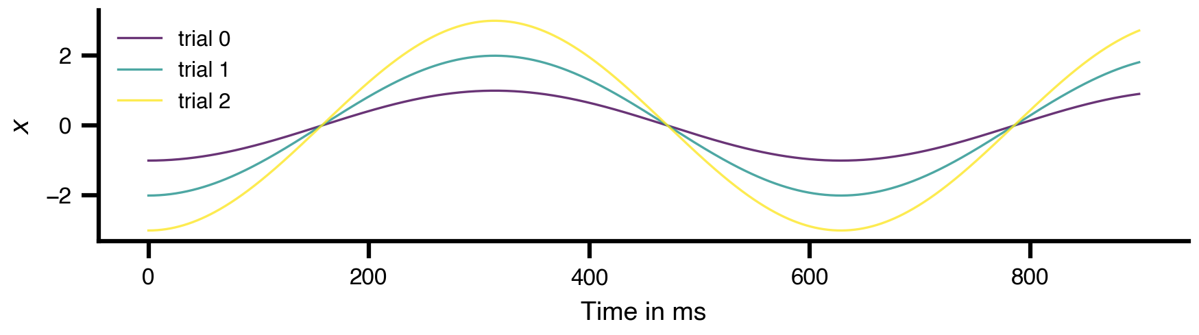
This is still the same spring object. Only the starting state changes.

1.5 Phase Space: The Geometry of the Flow

A time series shows one coordinate as a function of time. A phase portrait shows the full state \((x, v)\). This is the geometry-first view used in nonlinear dynamics and in phase-plane neuroscience.

For the undamped spring, the trajectories are closed loops because energy is conserved. The vector field is shared by every trajectory; only the initial condition changes.

from tvbo.datamodel.schema import Range
fig, ax = plt.subplots()
spring.state_variables['x'].domain = Range(lo=-5, hi=5)
spring.state_variables['v'].domain = Range(lo=-.05, hi=.05)
spring.plot("x", "v", kind="vectorfield", ax=ax)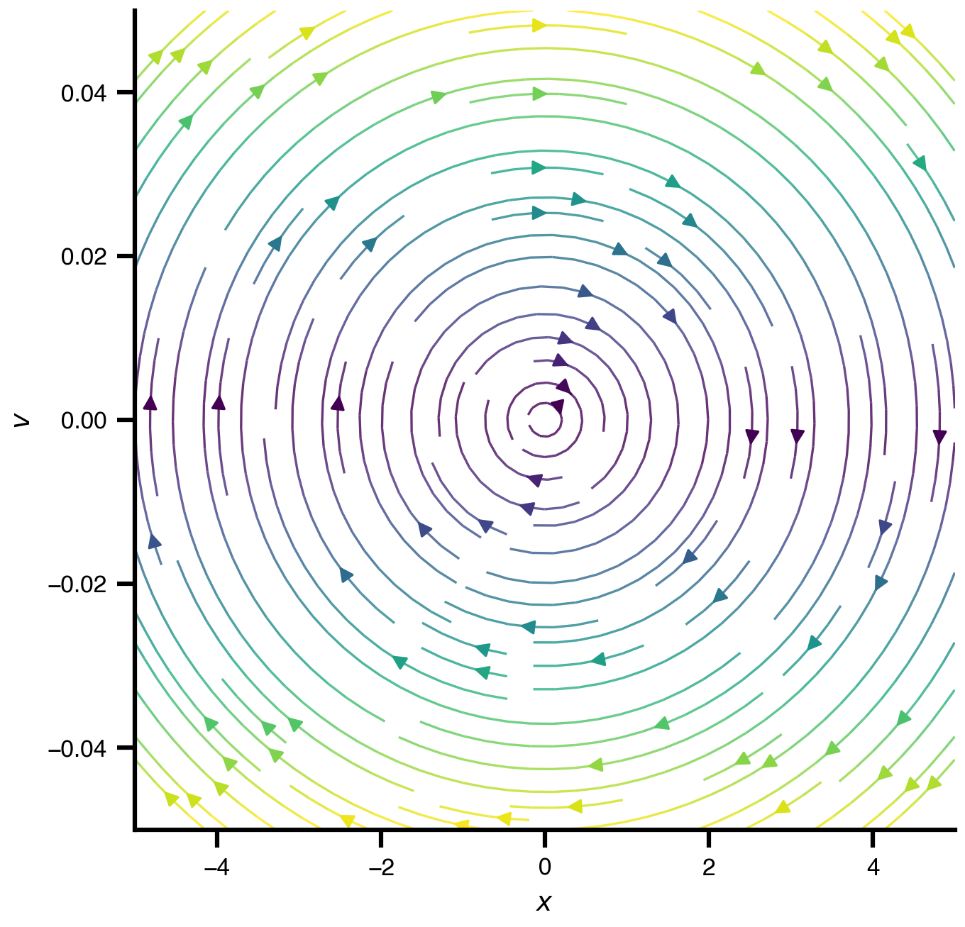

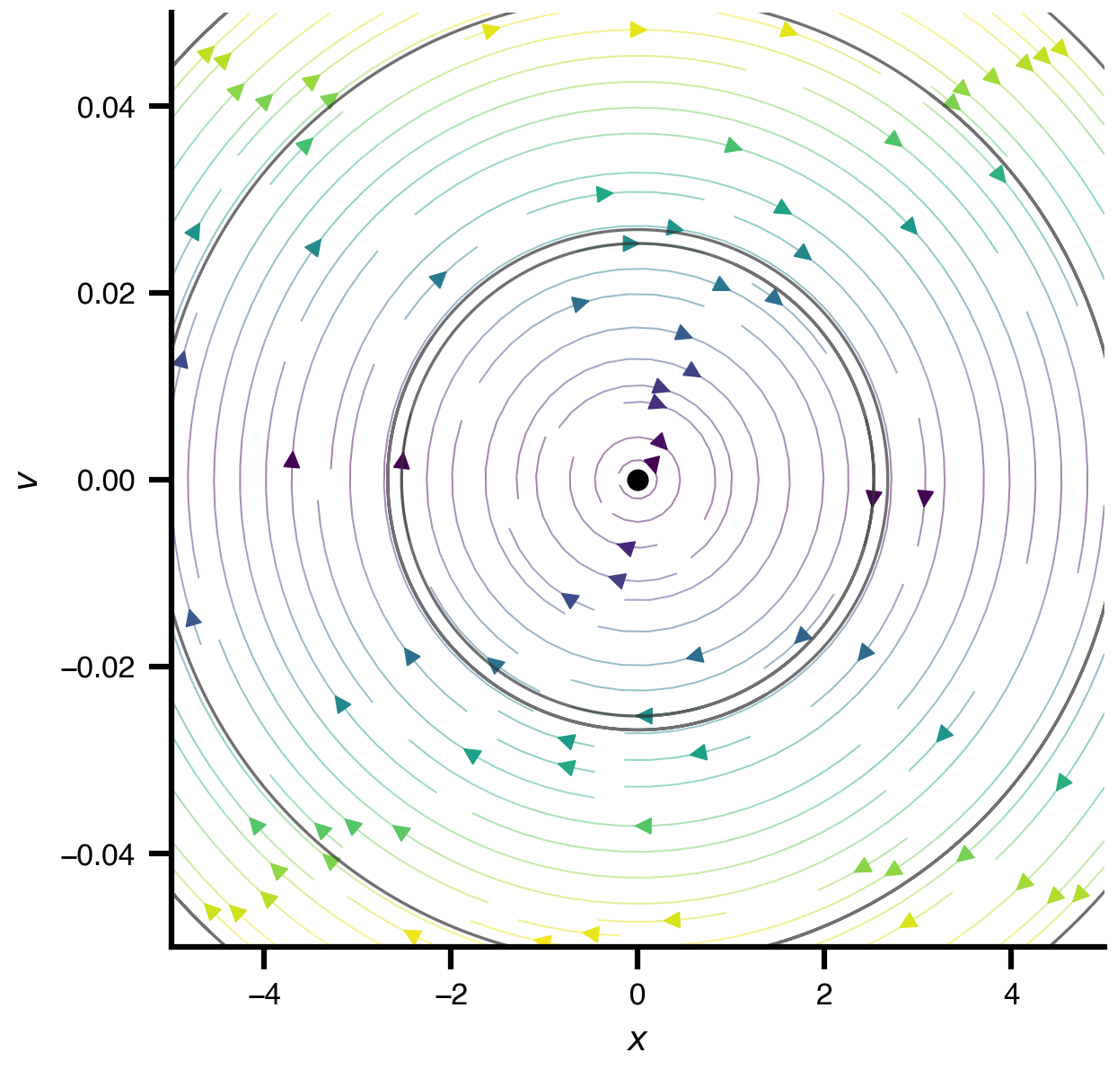
TVBO can also draw the phase plane directly, including vector field, nullclines, fixed points, and sample trajectories.

spring.plot(
    "x",
    "v",
    kind="phaseplane",
    duration=900.0,
    dt=1.0,
    n_trajectories=4,
    show_nullclines=False,
)

1.6 Parameters: Changing the System Itself

Parameters are different from initial conditions. Initial conditions choose where a trajectory begins; parameters reshape the vector field.

Here we vary the mass \(m\) while keeping \(k\), \(x_0\), and \(v_0\) fixed. Heavier mass means more inertia, so the oscillation is slower.

mass_experiment = SimulationExperiment(dynamics=spring)
mass_experiment.integration.duration = 1200.0
mass_experiment.integration.step_size = 1.0

mass_experiment.dynamics.state_variables["x"].initial_value = -2.0
mass_experiment.dynamics.state_variables["v"].initial_value = 0.0

mass_experiment.explorations["mass_sweep"] = Exploration(
    name="mass_sweep",
    space=ExplorationAxis(parameter="m", explored_values=[0.5, 1.0, 2.0]),
)

mass_result = mass_experiment.run("tvboptim")
mass_result.explorations["mass_sweep"].plot(overlay=True)

============================================================
STEP 1: Running simulation...
============================================================
  Simulation period: 1200.0 ms, dt: 1.0 ms
  Transient period: 0.0 ms
  Simulation complete.

============================================================
STEP 2: Running explorations...
============================================================
  > mass_sweep
  Explorations complete.

============================================================
Experiment complete.
============================================================

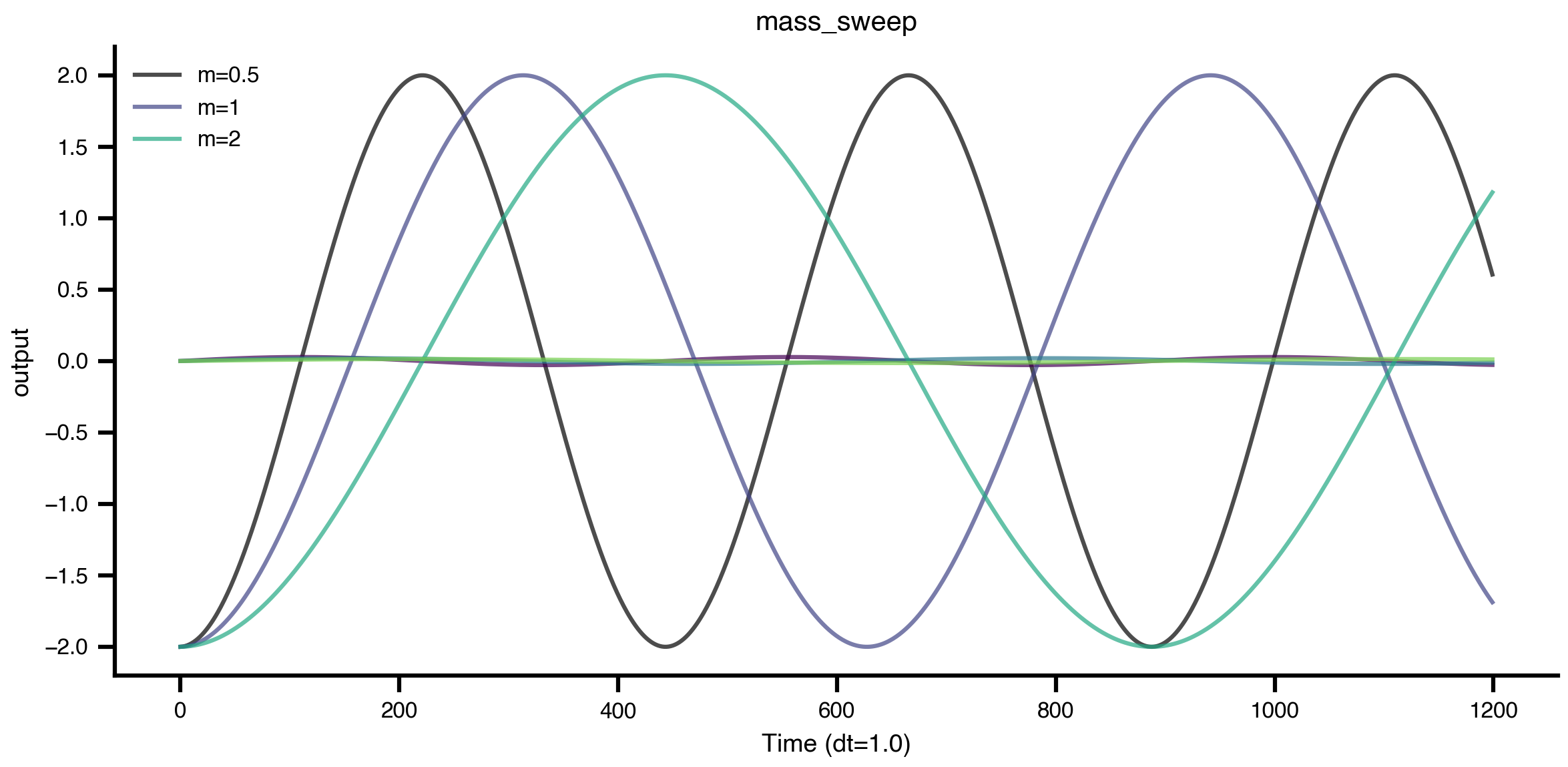
The sweep is part of the experiment specification. That is the pattern we want later: the metadata describes the exploration, and tvboptim executes it.

1.7 Toward Realism: Damping and Load

The ideal spring never loses energy. Real systems usually do. We can specify a second TVBO model by adding a damping term and a constant load:

\[ \dot{x} = v, \qquad \dot{v} = -\frac{k}{m}x - \frac{c}{m}v + g_{\mathrm{eff}}. \]

The damping term changes the transient. The load shifts the equilibrium from \(x = 0\) to

\[ x^* = \frac{m g_{\mathrm{eff}}}{k}. \]

damped_spring = Dynamics(
    name="DampedLoadedSpringMass",
    description="Spring-mass oscillator with damping and a constant load.",
    state_variables={
        "x": {
            "description": "Displacement from equilibrium",
            "unit": "m",
            "equation": {"rhs": "v"},
            "initial_value": 2.0,
        },
        "v": {
            "description": "Velocity",
            "unit": "m_per_s",
            "equation": {"rhs": "-(k/m) * x - (c/m) * v + g_eff"},
            "initial_value": 0.0,
        },
    },
    parameters={
        "k": {"description": "Spring stiffness", "unit": "N_per_m", "value": 0.0001},
        "m": {"description": "Mass", "unit": "kg", "value": 1.0},
        "c": {"description": "Damping coefficient", "unit": "kg_per_s", "value": 0.006},
        "g_eff": {"description": "Constant effective load", "unit": "m_per_s2", "value": 0.00015},
    },
)

Markdown(damped_spring.render("markdown"))

DampedLoadedSpringMass

Spring-mass oscillator with damping and a constant load.

autonomous: True; modes: 1; state variables: 2; parameters: 4.

State Equations

\[ \dot{x} = v \] \[ \dot{v} = g_{eff} - \frac{c*v}{m} - \frac{k*x}{m} \]

State Variables

Variable	Initial Value	Unit	Equation	Domain / Sampling	Flags	Description
\(x\)	2.0	\(\mathrm{m}\)	differential (order 1)	—	VOI, recorded	Displacement from equilibrium
\(v\)	0.0	\(\frac{\mathrm{m}}{\mathrm{s}}\)	differential (order 1)	—	VOI, recorded	Velocity

Parameters

Parameter	Value	Default	Unit	Domain / Sampling	Flags	Description
\(k\)	0.0001	—	\(\frac{\mathrm{N}}{\mathrm{m}}\)	—	—	Spring stiffness
\(m\)	1.0	—	\(\mathrm{kg}\)	—	—	Mass
\(c\)	0.006	—	\(\frac{\mathrm{kg}}{\mathrm{s}}\)	—	—	Damping coefficient
\(g_{eff}\)	0.00015	—	\(\frac{\mathrm{m}}{\mathrm{s}^2}\)	—	—	Constant effective load

damped_experiment = SimulationExperiment(dynamics=damped_spring)
damped_experiment.integration.duration = 1800.0
damped_experiment.integration.step_size = 1.0

damped_result = damped_experiment.run("tvboptim")
fig = damped_result.integration.plot()
fig.suptitle("Damped oscillator state variables")
fig

============================================================
STEP 1: Running simulation...
============================================================
  Simulation period: 1800.0 ms, dt: 1.0 ms
  Transient period: 0.0 ms
  Simulation complete.

============================================================
Experiment complete.
============================================================

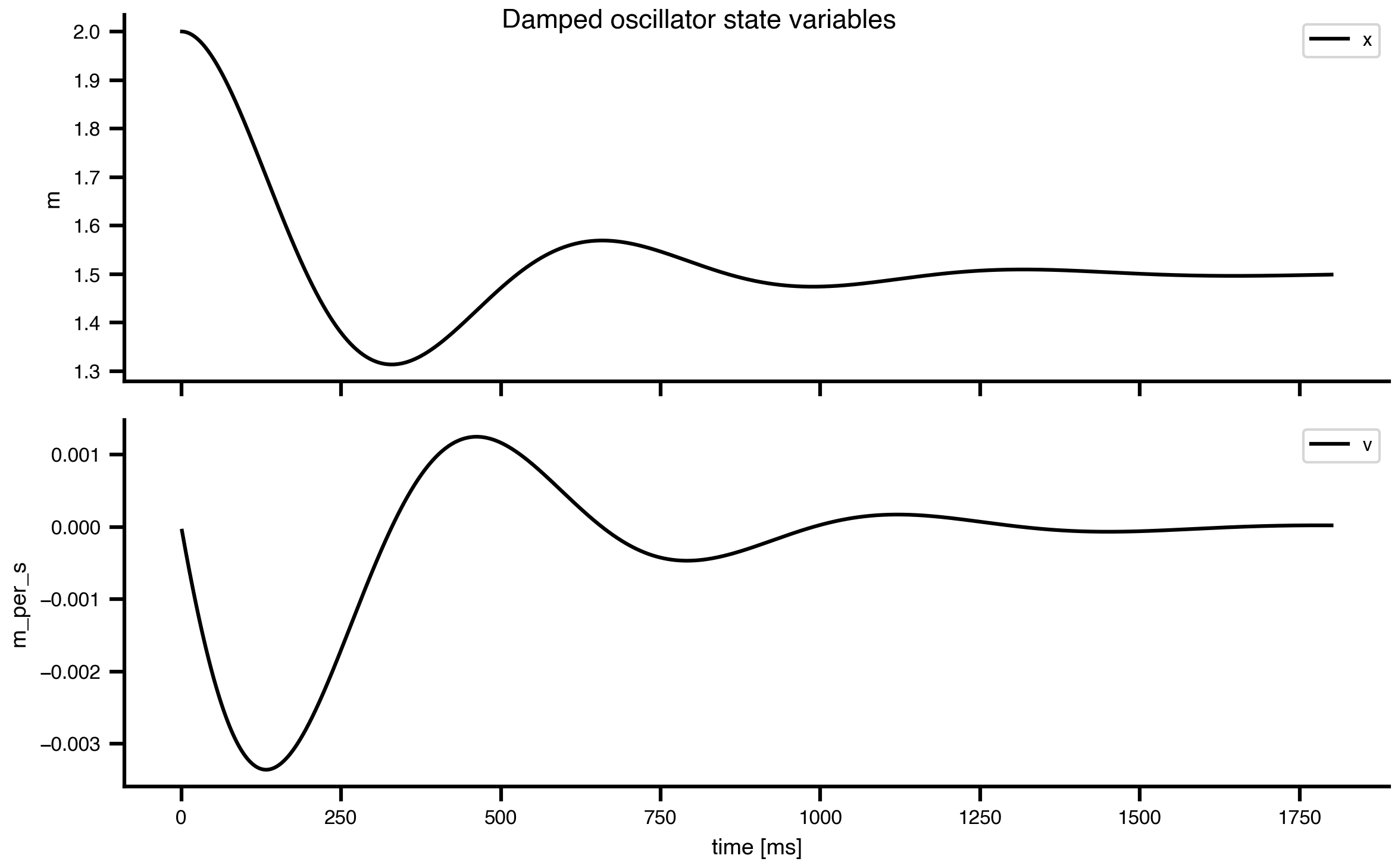
In phase space, damping turns closed loops into spirals. The constant load moves the final equilibrium to \(x^* = m g_{\mathrm{eff}} / k\).

damped_initial_conditions = np.array([
    [-2.5, 0.0],
    [-1.5, 0.015],
    [2.5, -0.01],
])

damped_spring.state_variables['x'].domain = Range(lo=-5, hi=5)
damped_spring.state_variables['v'].domain = Range(lo=-.05, hi=.05)

fig, ax = plt.subplots(figsize=(5.2, 4.8))

damped_spring.plot("x", "v", kind="vectorfield", ax=ax, alpha=0.35, grid_n=24, stream=True)
damped_spring.plot(
    "x",
    "v",
    kind="phase",
    ax=ax,
    duration=1800.0,
    dt=1.0,
    n_trials=len(damped_initial_conditions),
    u_0=damped_initial_conditions,
    cmap="plasma",
    lw=1.5,
)

x_equilibrium = damped_spring.parameters["m"].value * damped_spring.parameters["g_eff"].value / damped_spring.parameters["k"].value
ax.plot(x_equilibrium, 0.0, "o", color="C3", ms=7, mec="white", mew=1.0, zorder=10)
ax.set_title("Damping turns closed loops into spirals")
fig.tight_layout()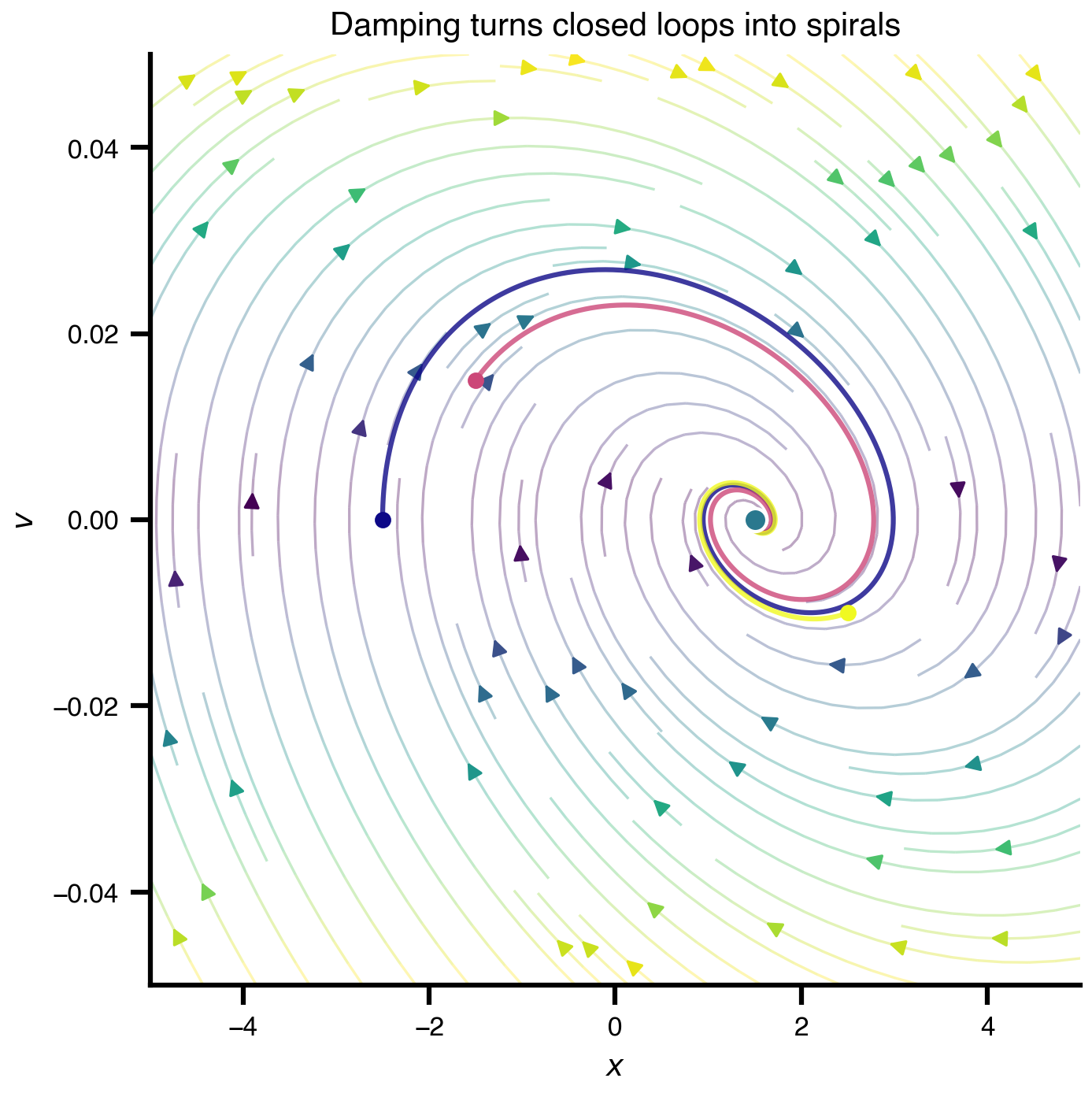

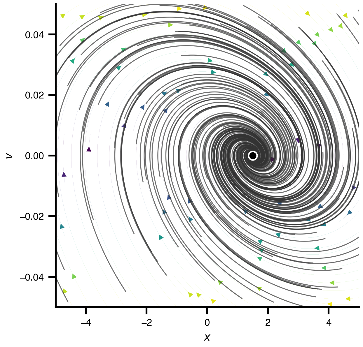
For a broader qualitative picture, let TVBO add sample trajectories on top of the damped phase plane.

damped_spring.plot(
    "x",
    "v",
    kind="phaseplane",
    duration=1800.0,
    dt=1.0,
    n_trajectories=100,
    show_nullclines=False,
    lw=0.1
)

1.8 Connection to TVBO Documentation

The spring example is intentionally simple, but each piece maps directly to the main TVBO documentation topics.

Concept in this notebook	TVBO object or method	Why it matters later
Equations and parameters	Dynamics	Neural mass and oscillator models use the same schema.
Full experiment execution	SimulationExperiment.run("tvboptim")	The experiment combines dynamics, integration, networks, observations, algorithms, and continuations.
Named output	result.integration.data	Results are xarray objects, so analysis should use named dimensions like time, variable, and node.
Parameter sweeps	Exploration, ExplorationAxis	Parameter scans become declarative experiment metadata.
Damping and load	Model specification	More realistic assumptions are added by changing equations and parameters, not by changing the execution workflow.

1.9 From Spring-Mass to Neural Mass Models

The next workshop section moves from a physical toy system to neural mass models. The TVBO database already stores many such models with the same structure: state variables, parameters, equations, and metadata.

neural_mass_models = Dynamics.list_db(model_type="neural_mass")
neural_mass_models[:8]

['CakanObermayer',
 'Epileptor3DStefanescuMcDonald',
 'GastSchmidtKnosche_SD',
 'GastSchmidtKnosche_SF',
 'Hopfield',
 'JansenRit',
 'JansenRit1995',
 'LarterBreakspear']

jansen_rit = Dynamics.from_db("JansenRit")
print("state variables:", list(jansen_rit.state_variables))
print("first parameters:", list(jansen_rit.parameters)[:8])

state variables: ['y0', 'y1', 'y2', 'y3', 'y4', 'y5']
first parameters: ['A', 'B', 'J', 'a_1', 'a_2', 'a_3', 'a_4', 'a']

This is the key bridge: the spring has \((x, v)\), while a neural mass model has variables such as membrane potentials, firing-rate transforms, or synaptic gating variables. But the TVBO workflow remains the same:

1. Choose or define Dynamics.
2. Put it in a SimulationExperiment.
3. Run the experiment.
4. Plot and analyze the result.

1.9.1 TASK: Run and Plot Simple Single-Node SimulationExperiment with JansenRit Model