Code
import numpy as np
import matplotlib.pyplot as plt
from tvbo import Dynamics, Continuation, SimulationExperiment
from tvbo.datamodel.schema import Exploration, ExplorationAxisexp.run(backend) call.Bifurcation analysis tells us how the qualitative behaviour of a model changes when we move a parameter. In TVBO every example below is just inline YAML + plotting — no Fortran files, no scratch directories.
import numpy as np
import matplotlib.pyplot as plt
from tvbo import Dynamics, Continuation, SimulationExperiment
from tvbo.datamodel.schema import Exploration, ExplorationAxisThe simplest dynamical system is
\[ \dot x = a\,x, \qquad x(0) = x_0, \qquad x(t) = x_0\,e^{a t}. \]
For \(a < 0\) the origin is a stable fixed point, for \(a > 0\) it is unstable, and \(a = 0\) is the prototype of a bifurcation.
LIN = """
name: LinearScalar
parameters:
  a:
    name: a
    value: 1.0
state_variables:
  x:
    name: x
    equation:
      lhs: Derivative(x, t)
      rhs: a*x
    initial_value: 1.0
"""

exp_lin = SimulationExperiment(dynamics=Dynamics.from_string(LIN))
exp_lin.integration.duration = 4
exp_lin.integration.step_size = 1e-3
exp_lin.explorations["a_sweep"] = Exploration(
    name="a_sweep",
    space=ExplorationAxis(parameter="a", explored_values=[-1.0, -0.5, 0.0, 0.5, 1.0]),
)
exp_lin.run("tvboptim").explorations["a_sweep"].plot(overlay=True)
============================================================
STEP 1: Running simulation...
============================================================
  Simulation period: 4.0 ms, dt: 0.001 ms
  Transient period: 0.0 ms
  Simulation complete.

============================================================
STEP 2: Running explorations...
============================================================
  > a_sweep
  Explorations complete.

============================================================
Experiment complete.
============================================================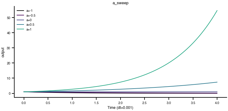
The slope at \(t = 0\) equals \(a\) — its sign decides growth vs. decay. For nonlinear systems \(\dot x = f(x)\), stability of an equilibrium \(x^*\) is governed by the Jacobian eigenvalues \(J = \partial f/\partial x|_{x^*}\). Everything that follows is built from this idea.
For \(\dot{\vec x} = A\vec x\) in 2D, the eigenvalues of \(A\) classify the origin. TVBO’s kind="phaseplane" overlays the vector field with both nullclines and the detected fixed points.
Each system below is a complete, copy-pastable YAML. We feed it directly to Dynamics.from_string — no helper functions, no string interpolation.
SADDLE = """
name: Saddle
state_variables:
  x1:
    name: x1
    domain:
      lo: -2.0
      hi: 2.0
    equation:
      lhs: Derivative(x1, t)
      rhs: x1 - x2
    initial_value: 1.0
  x2:
    name: x2
    domain:
      lo: -2.0
      hi: 2.0
    equation:
      lhs: Derivative(x2, t)
      rhs: -x1 - x2
    initial_value: 1.0
"""

STABLE_NODE = """
name: StableNode
state_variables:
  x1:
    name: x1
    domain:
      lo: -2.0
      hi: 2.0
    equation:
      lhs: Derivative(x1, t)
      rhs: -2*x1
    initial_value: 1.0
  x2:
    name: x2
    domain:
      lo: -2.0
      hi: 2.0
    equation:
      lhs: Derivative(x2, t)
      rhs: -x2
    initial_value: 1.0
"""

STABLE_FOCUS = """
name: StableFocus
state_variables:
  x1:
    name: x1
    domain:
      lo: -2.0
      hi: 2.0
    equation:
      lhs: Derivative(x1, t)
      rhs: -0.3*x1 - x2
    initial_value: 1.0
  x2:
    name: x2
    domain:
      lo: -2.0
      hi: 2.0
    equation:
      lhs: Derivative(x2, t)
      rhs: x1 - 0.3*x2
    initial_value: 1.0
"""

CENTRE = """
name: Centre
state_variables:
  x1:
    name: x1
    domain:
      lo: -2.0
      hi: 2.0
    equation:
      lhs: Derivative(x1, t)
      rhs: -x2
    initial_value: 1.0
  x2:
    name: x2
    domain:
      lo: -2.0
      hi: 2.0
    equation:
      lhs: Derivative(x2, t)
      rhs: x1
    initial_value: 1.0
"""

CASES = [
    ("Saddle",       SADDLE),
    ("Stable node",  STABLE_NODE),
    ("Stable focus", STABLE_FOCUS),
    ("Centre",       CENTRE),
]

fig, axes = plt.subplots(2, 2, figsize=(8, 6.5))
for ax, (label, yml) in zip(axes.flat, CASES):
    dyn = Dynamics.from_string(yml)
    dyn.plot("x1", "x2", kind="vectorfield", ax=ax,
             grid_n=20, n_trajectories=3, duration=15)
    ax.set_title(label, fontsize=10)
plt.tight_layout(); plt.show()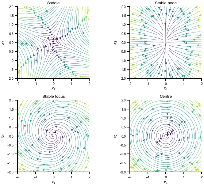
Bifurcations occur when an eigenvalue of \(A\) — or, locally, of the Jacobian — crosses the imaginary axis as a parameter is varied.
We cover the canonical scalar bifurcations and let TVBO continue the equilibrium branch bidirectionally. Each example is a self-contained YAML pair (Dynamics + Continuation) passed straight into from_string.
Two equilibria collide and annihilate at \(a = 0\). Beyond the fold no attractor survives. This is the prototype for regime shifts.
SADDLE_NODE = """
name: SaddleNode
parameters:
  a:
    name: a
    value: 1.0
state_variables:
  x:
    name: x
    domain:
      lo: -2.0
      hi: 2.0
    equation:
      lhs: Derivative(x, t)
      rhs: a - x**2
    initial_value: 1.0
"""

SADDLE_NODE_CONT = """
name: saddle_node_cont
dynamics: SaddleNode
free_parameters:
  - name: a
    domain:
      lo: -2.0
      hi: 2.0
max_steps: 400
ds: 0.01
bothside: true
"""

exp_sn = SimulationExperiment(
    dynamics=Dynamics.from_string(SADDLE_NODE),
    continuations=[Continuation.from_string(SADDLE_NODE_CONT)],
)
exp_sn.run("bifurcationkit.jl").continuations["saddle_node_cont"].plot(VOI="x")
plt.show()
CT: 0.428738 seconds (806.41 k allocations: 39.307 MiB, 99.90% compilation time)
CT: 0.000342 seconds (7.60 k allocations: 318.734 KiB)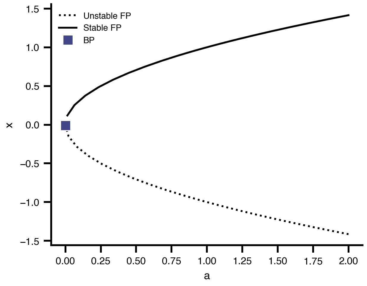
exp_sn.run('tvboptim').plot()
============================================================
STEP 1: Running simulation...
============================================================
  Simulation period: 1000.0 ms, dt: 0.01220703125 ms
  Transient period: 0.0 ms
  Simulation complete.

============================================================
Experiment complete.
============================================================
A small constant tilt unfolds the pitchfork into two saddle-nodes framing a bistable region. Sweeping \(a\) up then down traces a memory loop.
HYSTERESIS = """
name: Hysteresis
parameters:
  a:
    name: a
    value: 1.0
state_variables:
  x:
    name: x
    domain:
      lo: -2.0
      hi: 2.0
    equation:
      lhs: Derivative(x, t)
      rhs: a + x - x**3
    initial_value: 1.0
"""

HYSTERESIS_CONT = """
name: hysteresis_cont
dynamics: Hysteresis
free_parameters:
  - name: a
    domain:
      lo: -1.5
      hi: 1.5
max_steps: 400
ds: 0.01
bothside: true
"""

exp_hy = SimulationExperiment(
    dynamics=Dynamics.from_string(HYSTERESIS),
    continuations=[Continuation.from_string(HYSTERESIS_CONT)],
)
exp_hy.run("bifurcationkit.jl").continuations["hysteresis_cont"].plot(VOI="x")
plt.show()
CT: 0.447745 seconds (805.92 k allocations: 39.244 MiB, 99.90% compilation time)
CT: 0.000526 seconds (10.88 k allocations: 451.875 KiB)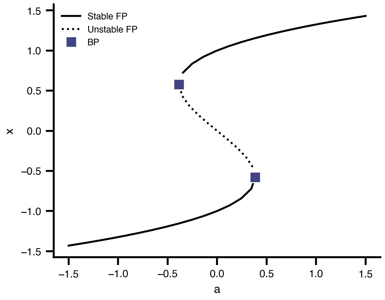
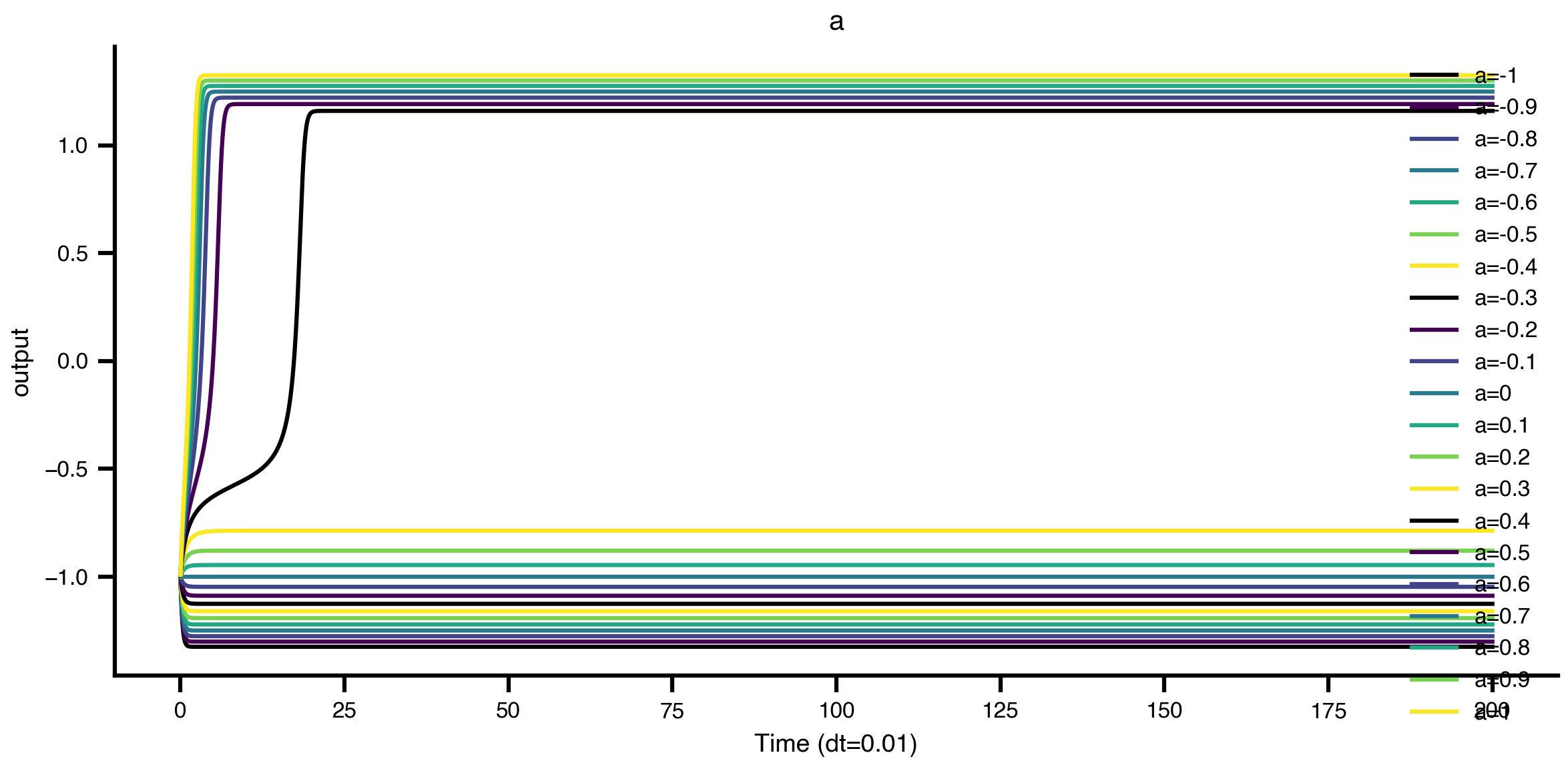
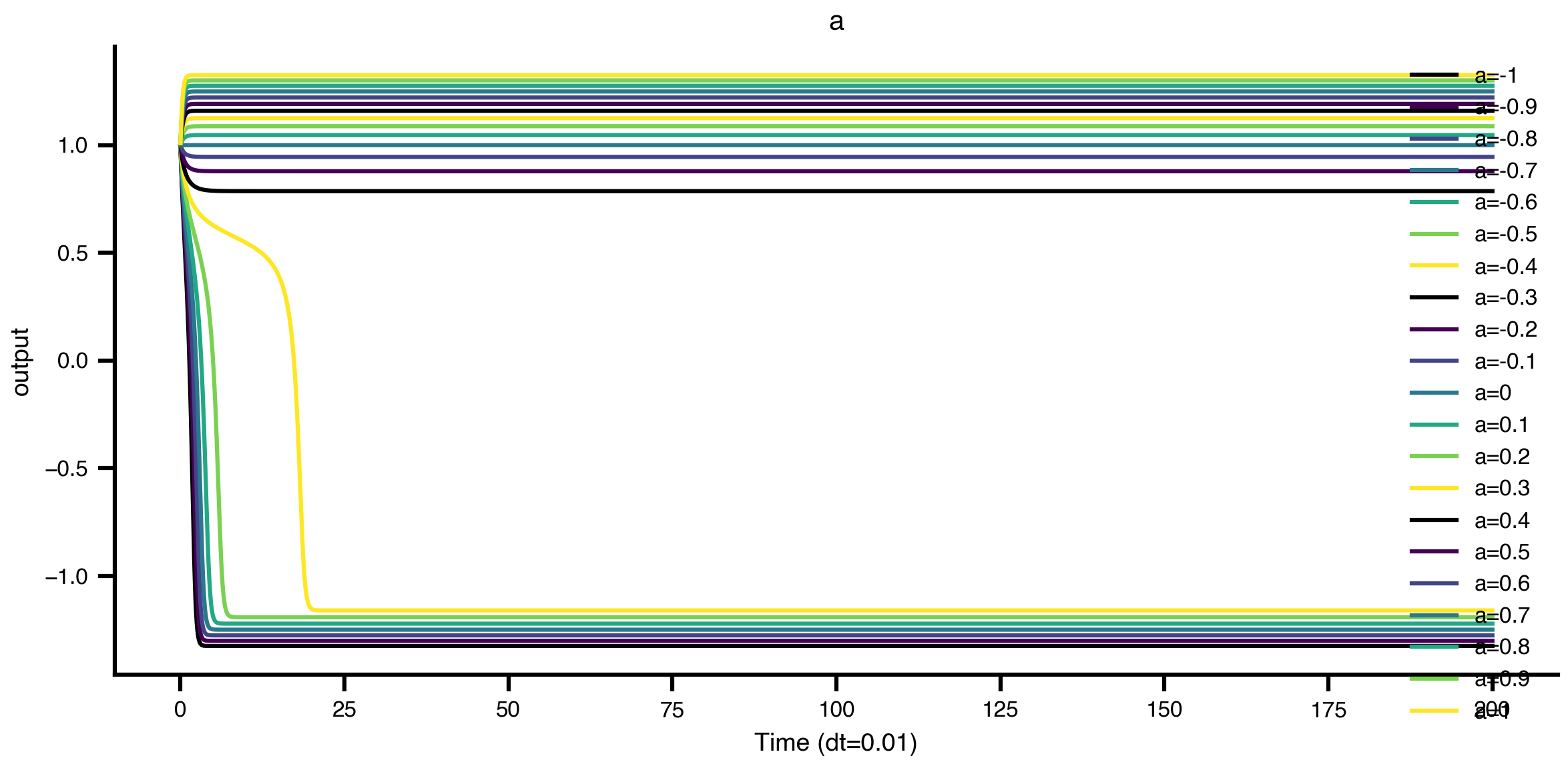
Two Explorations over \(a\) — one starting from \(x_0 = -1\), one from \(x_0 = +1\) — expose the bistable region: for the same \(a\), each initial condition lands on a different attractor.
dyn_lo = Dynamics.from_string(HYSTERESIS)
dyn_lo.state_variables["x"].initial_value = -1.0
exp_hy_lo = SimulationExperiment(dynamics=dyn_lo)
exp_hy_lo.integration.duration = 200
exp_hy_lo.integration.step_size = 0.01
exp_hy_lo.explorations["a"] = Exploration(
    name="a",
    space=ExplorationAxis(parameter="a", explored_values=list(np.linspace(-1.0, 1.0, 21))),
)
exp_hy_lo.run("tvboptim").explorations["a"].plot(overlay=True)
============================================================
STEP 1: Running simulation...
============================================================
  Simulation period: 200.0 ms, dt: 0.01 ms
  Transient period: 0.0 ms
  Simulation complete.

============================================================
STEP 2: Running explorations...
============================================================
  > a
  Explorations complete.

============================================================
Experiment complete.
============================================================
dyn_hi = Dynamics.from_string(HYSTERESIS)
dyn_hi.state_variables["x"].initial_value = 1.0
exp_hy_hi = SimulationExperiment(dynamics=dyn_hi)
exp_hy_hi.integration.duration = 200
exp_hy_hi.integration.step_size = 0.01
exp_hy_hi.explorations["a"] = Exploration(
    name="a",
    space=ExplorationAxis(parameter="a", explored_values=list(np.linspace(-1.0, 1.0, 21))),
)
exp_hy_hi.run("tvboptim").explorations["a"].plot(overlay=True)
============================================================
STEP 1: Running simulation...
============================================================
  Simulation period: 200.0 ms, dt: 0.01 ms
  Transient period: 0.0 ms
  Simulation complete.

============================================================
STEP 2: Running explorations...
============================================================
  > a
  Explorations complete.

============================================================
Experiment complete.
============================================================
In 2D, a Hopf bifurcation occurs when a pair of complex-conjugate eigenvalues crosses the imaginary axis. A stable focus turns into an unstable focus surrounded by a stable limit cycle of radius \(\sqrt a\).
\[ \dot x_1 = (a - x_1^2 - x_2^2)\,x_1 - w\,x_2, \qquad \dot x_2 = (a - x_1^2 - x_2^2)\,x_2 + w\,x_1. \]
HOPF = r"""
name: HopfNF
parameters:
  a:
    name: a
    value: 0.5
  w:
    name: w
    value: 1.0
state_variables:
  x1:
    name: x1
    domain:
      lo: -2.0
      hi: 2.0
    equation:
      lhs: Derivative(x1, t)
      rhs: (a - x1**2 - x2**2)*x1 - w*x2
    initial_value: 0.0
  x2:
    name: x2
    domain:
      lo: -2.0
      hi: 2.0
    equation:
      lhs: Derivative(x2, t)
      rhs: (a - x1**2 - x2**2)*x2 + w*x1
    initial_value: 0.0
"""

CONT_HOPF = """
name: hopf_in_a
dynamics: HopfNF
free_parameters:
  - name: a
    domain:
      lo: -2.0
      hi: 2.0
max_steps: 400
ds: 0.01
bothside: true
branches:
  - name: po_from_hopf
    source_point: "hopf:all"
    bothside: true
"""

dyn  = Dynamics.from_string(HOPF)
cont = Continuation.from_string(CONT_HOPF)
exp_hopf = SimulationExperiment(dynamics=dyn, continuations=[cont])
hopf = exp_hopf.run("bifurcationkit.jl").continuations["hopf_in_a"]
CT: 0.405260 seconds (796.98 k allocations: 39.072 MiB, 99.92% compilation time)
CT: 0.000170 seconds (2.14 k allocations: 191.859 KiB)
CT: 2.778990 seconds (3.25 M allocations: 518.271 MiB, 3.43% gc time, 94.47% compilation time)
CT: 0.155940 seconds (226.88 k allocations: 390.487 MiB, 9.05% gc time)The 2D bifurcation diagram (MIN/MAX envelope of the limit cycle):
hopf.plot(VOI="x1"); plt.show()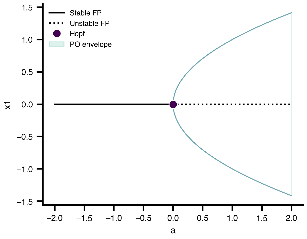
The 3D view shows the equilibrium spine, the Hopf point, and the limit-cycle tube whose radius grows like \(\sqrt a\):
hopf.plot_3d(VOI="x1"); plt.show()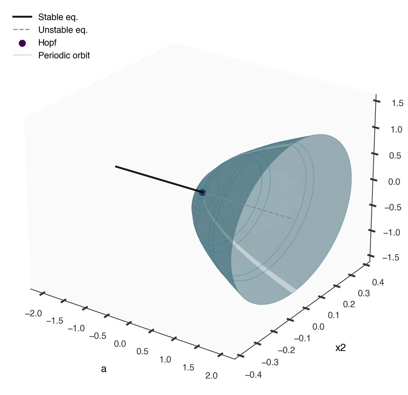
The backend (bifurcationkit.jl) tracks equilibria \(f(x, a) = 0\) along arclength \(s\) instead of along \(a\) directly. A predictor-corrector scheme (tangent extrapolation + Newton on the augmented system) walks past folds where \(J\) becomes singular. Bifurcations are flagged by sign changes in test functions (\(\det J\) for folds, \(\mathrm{Re}\,\lambda\) for Hopf, etc.). At a branch point the corrector restarts in the eigenvector direction. This is branch switching, and in TVBO it is requested declaratively:
branches:
  - name: po_from_hopf
    source_point: "hopf:all"
Task: run the following example with and without the branches attributes
The same Continuation API drives a TVB neural-mass model. We sweep the external input \(I\) and let TVBO continue periodic orbits from every detected Hopf point.
model = Dynamics.from_ontology("Generic2dOscillator")

cont = Continuation.from_string("""
name: g2d_in_I
dynamics: Generic2dOscillator
free_parameters:
  - name: I
    domain:
      lo: -10.0
      hi: 20.0
max_steps: 500
ds: 0.05
bothside: true
# branches:
#   - name: po_from_hopf
#     source_point: "hopf:all"
#     bothside: true
""")

exp_g2d = SimulationExperiment(dynamics=model, continuations=[cont])
g2d = exp_g2d.run("bifurcationkit.jl").continuations["g2d_in_I"]
g2d.plot(VOI="V"); plt.show()
CT: 0.427159 seconds (841.83 k allocations: 41.830 MiB, 99.42% compilation time)
CT: 0.000874 seconds (15.79 k allocations: 1.171 MiB)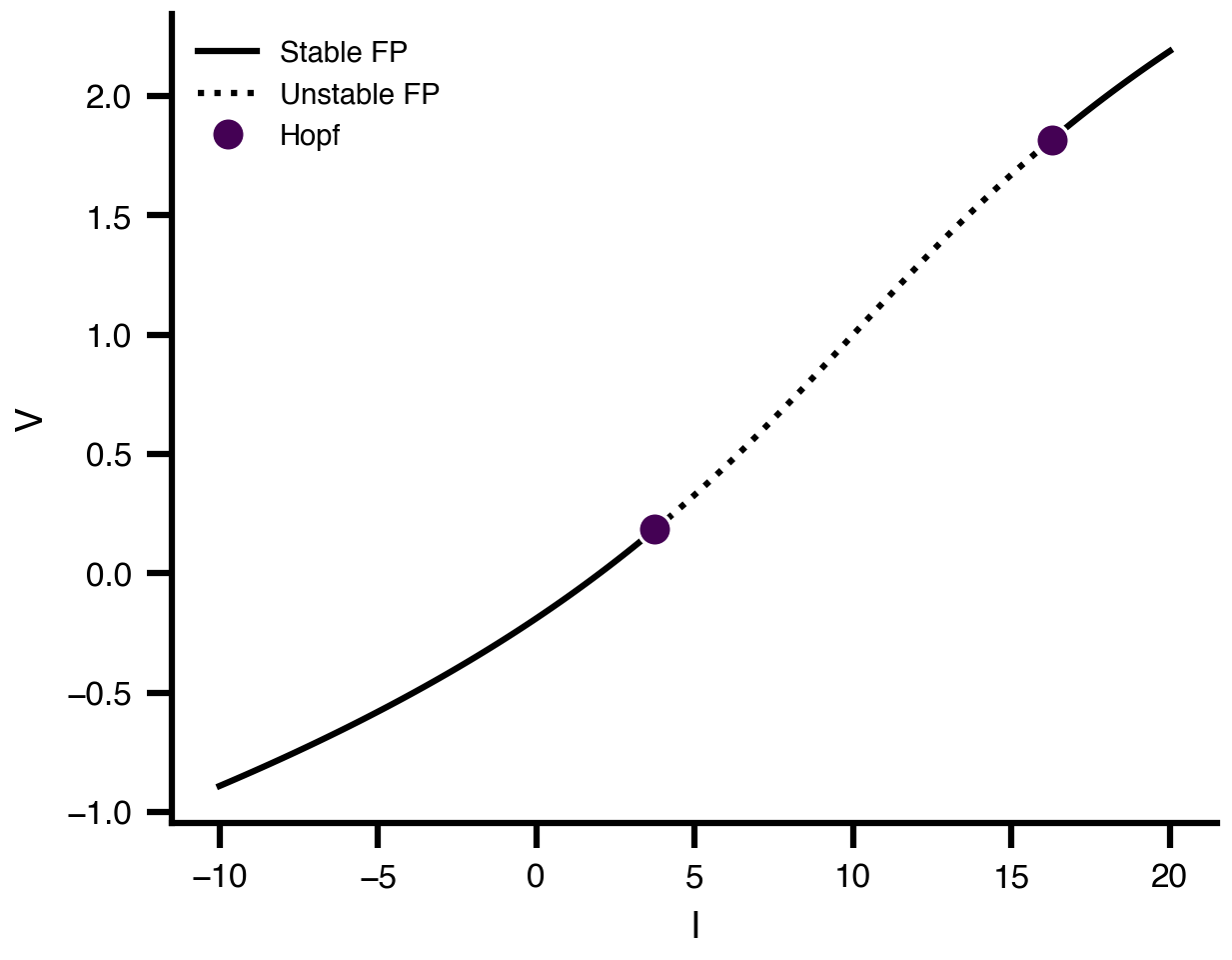
g2d.plot_3d(VOI="V"); plt.show()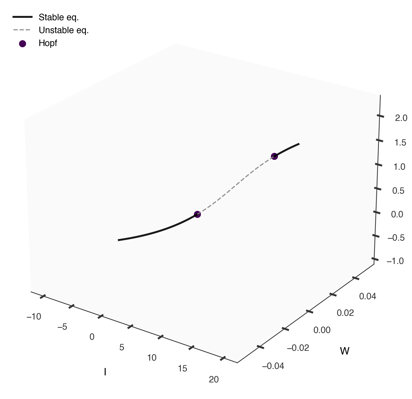
Reading the diagram: stable branches → resting / persistent activity; limit cycles → oscillatory regime; folds → abrupt regime shifts (e.g. seizure onset). The same machinery applied to a whole-brain network predicts where the collective dynamics changes regime as global coupling or input is varied.
rhs: (a - r**2)*x1 - w*x2 + I0. Sweep I0 instead of a. What kind of bifurcation do you see?Generic2dOscillator, replace I by b as the free parameter. Where are the Hopf points now?