This tutorial demonstrates how to use TVB-Optim to fit functional connectivity (FC) data from resting-state fMRI. We use the Reduced Wong-Wang (RWW) neural mass model to simulate brain activity, convert it to BOLD signal using a hemodynamic response function, and optimize model parameters to match empirical FC patterns.
The workflow includes:
Building a whole-brain network with the RWW model
Simulating BOLD signal from neural activity
Computing functional connectivity from BOLD
Optimizing global and region-specific parameters to fit target FC
What you’ll learn
Concepts: how a neural mass model produces BOLD, what FC is and how it’s computed, why we exchange RMSE for correlation when judging fit quality.
TVB-Optim idioms: wrapping a value in Parameter(...) to mark it optimizable, setting .shape = (n_nodes,) to make a parameter regional, Space(..., mode="product") for grid exploration, and the @cache(...) decorator for skipping expensive reruns.
Workflow: grid exploration → global gradient fit → heterogeneous (per-region) fit, and how to read the resulting parameter landscape.
Environment Setup and Imports
# Set up environment# Note: XLA_FLAGS must be set BEFORE importing jax — it controls how many# virtual CPU devices JAX exposes. We expose N=8 here so that ParallelExecution# can map work over 8 devices later (see `n_pmap=8` in Parameter Exploration).import osimport timecpu =Trueif cpu: N =8 os.environ['XLA_FLAGS'] =f'--xla_force_host_platform_device_count={N}'# Import all required librariesimport numpy as npimport matplotlib.pyplot as pltimport matplotlib.patheffects as path_effectsimport jaximport jax.numpy as jnpimport copyimport optaxfrom scipy import io# Import from tvboptimfrom tvboptim.types import Parameter, Space, GridAxisfrom tvboptim.types.stateutils import show_parametersfrom tvboptim.utils import set_cache_path, cachefrom tvboptim.execution import ParallelExecution, SequentialExecutionfrom tvboptim.optim.optax import OptaxOptimizerfrom tvboptim.optim.callbacks import MultiCallback, DefaultPrintCallback, SavingCallback# Network dynamics importsfrom tvboptim.experimental.network_dynamics import Network, solve, preparefrom tvboptim.experimental.network_dynamics.dynamics.tvb import ReducedWongWang, WongWangExcInhfrom tvboptim.experimental.network_dynamics.coupling import LinearCoupling, FastLinearCouplingfrom tvboptim.experimental.network_dynamics.graph import DenseDelayGraph, DenseGraphfrom tvboptim.experimental.network_dynamics.solvers import Heunfrom tvboptim.experimental.network_dynamics.noise import AdditiveNoisefrom tvboptim.data import load_structural_connectivity, load_functional_connectivity# BOLD monitoringfrom tvboptim.observations.tvb_monitors.bold import Bold# Observation functionsfrom tvboptim.observations.observation import compute_fc, fc_corr, rmse# Set cache path for tvboptimset_cache_path("./rww")
We enable 64-bit precision to get reliable gradient information.
jax.config.update("jax_enable_x64", True)
2 Loading Structural Data and Target FC
We load the Desikan-Killiany parcellation structural connectivity and empirical functional connectivity from resting-state fMRI data.
Load structural connectivity and target FC
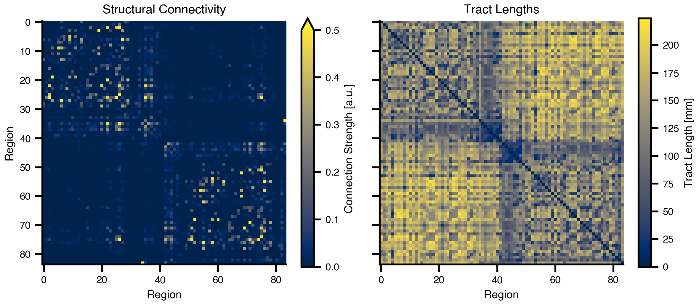
# Load structural connectivity with region labels# No delays for this model (instantaneous coupling)weights, lengths, region_labels = load_structural_connectivity(name="dk_average")# Normalize weights to [0, 1] rangeweights = weights / np.max(weights)n_nodes = weights.shape[0]# Load empirical functional connectivity as optimization targetfc_target = load_functional_connectivity(name="dk_average")
Figure 1: Structural connectivity matrices. Left: Normalized connection weights showing the strength of white matter connections between brain regions. Right: Tract lengths in millimeters representing the physical distance of fiber pathways.
3 The Reduced Wong-Wang Model
The Reduced Wong-Wang model is a biophysically-based neural mass model that describes the dynamics of NMDA-mediated synaptic gating. It captures the slow dynamics relevant for resting-state fMRI and has been widely used for modeling whole-brain functional connectivity.
The model describes the evolution of synaptic gating variable S:
where \(x = w \cdot J_N \cdot S + I_o + G \cdot c\) combines local recurrence (\(w\)), external input (\(I_o\)), and long-range coupling (\(G \cdot c\)), and \(H(x)\) is a sigmoidal transfer function.
We prepare the network for simulation and run an initial transient to reach a quasi-stationary state.
# Prepare simulation: compile model and initialize statet1 =90_000# Total simulation duration (ms) - 2 minutesdt =4.0# Integration timestep (ms)model, state = prepare(network, Heun(), t1=t1, dt=dt)# First simulation: run transient to reach quasi-stationary stateresult_init = model(state)# Update network with final state as new initial conditionsnetwork.update_history(result_init)model, state = prepare(network, Heun(), t1=t1, dt=dt)# Second simulation: quasi-stationary dynamicsresult = model(state)
6 Computing BOLD Signal
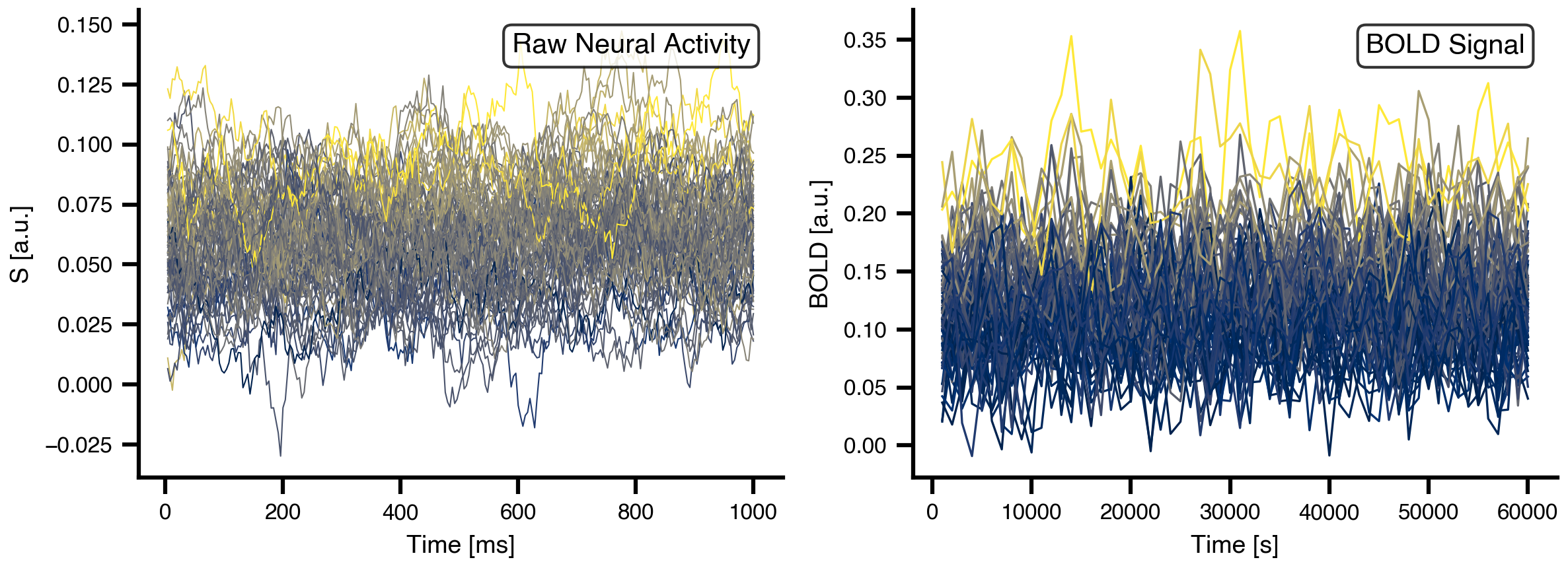
We convert the neural activity (synaptic gating S) to simulated BOLD signal using a hemodynamic response function. The BOLD monitor downsamples the neural activity and convolves it with a canonical HRF kernel.
# Create BOLD monitor with standard parametersbold_monitor = Bold( period=1000.0, # BOLD sampling period (1 TR = 1000 ms) downsample_period=4.0, # Intermediate downsampling matches dt voi=0, # Monitor first state variable (S) history=result_init # Use initial state as warm start)# Apply BOLD monitor to simulation resultbold_result = bold_monitor(result)
/var/folders/ym/9kw1g21j1nd7kwfn8c0z3st40000gn/T/ipykernel_33908/2955482924.py:2: DeprecationWarning: Bold is deprecated and will be removed in a future version. Use HRFBold (HRF convolution) or BalloonWindkesselBold (ODE integration) explicitly.
  bold_monitor = Bold(
Figure 2: Neural activity and BOLD signal time series. Left: Raw synaptic gating variable (S) showing fast neural dynamics over 1 second. Right: Simulated BOLD signal showing slow hemodynamic response over 60 seconds. Each line represents one brain region, colored by mean activity level.
7 Defining Observations and Loss
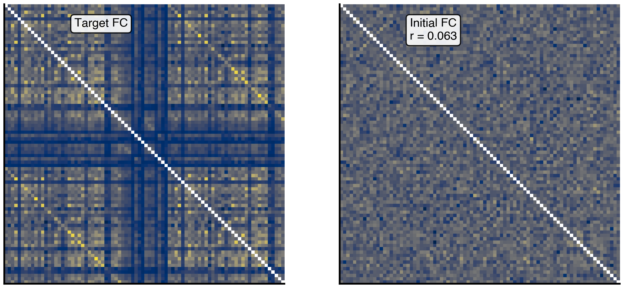
Functional connectivity (FC) measures the temporal correlation between BOLD signals from different brain regions. We define an observation function that simulates BOLD and computes FC, and a loss function that quantifies the mismatch with empirical FC.
def observation(state):"""Compute functional connectivity from simulated BOLD signal."""# Run simulation result = model(state)# Convert to BOLD bold = bold_monitor(result)# Compute FC, skipping first 20 TRs to avoid transient effects fc = compute_fc(bold, skip_t=20)return fcdef loss(state):"""Compute RMSE between simulated and empirical FC.""" fc = observation(state)return rmse(fc, fc_target)
Figure 3: Initial functional connectivity comparison. Left: Empirical FC from resting-state fMRI serving as optimization target. Right: Simulated FC from initial model parameters showing poor correlation with target (r = correlation coefficient between the two matrices).
8 Parameter Exploration
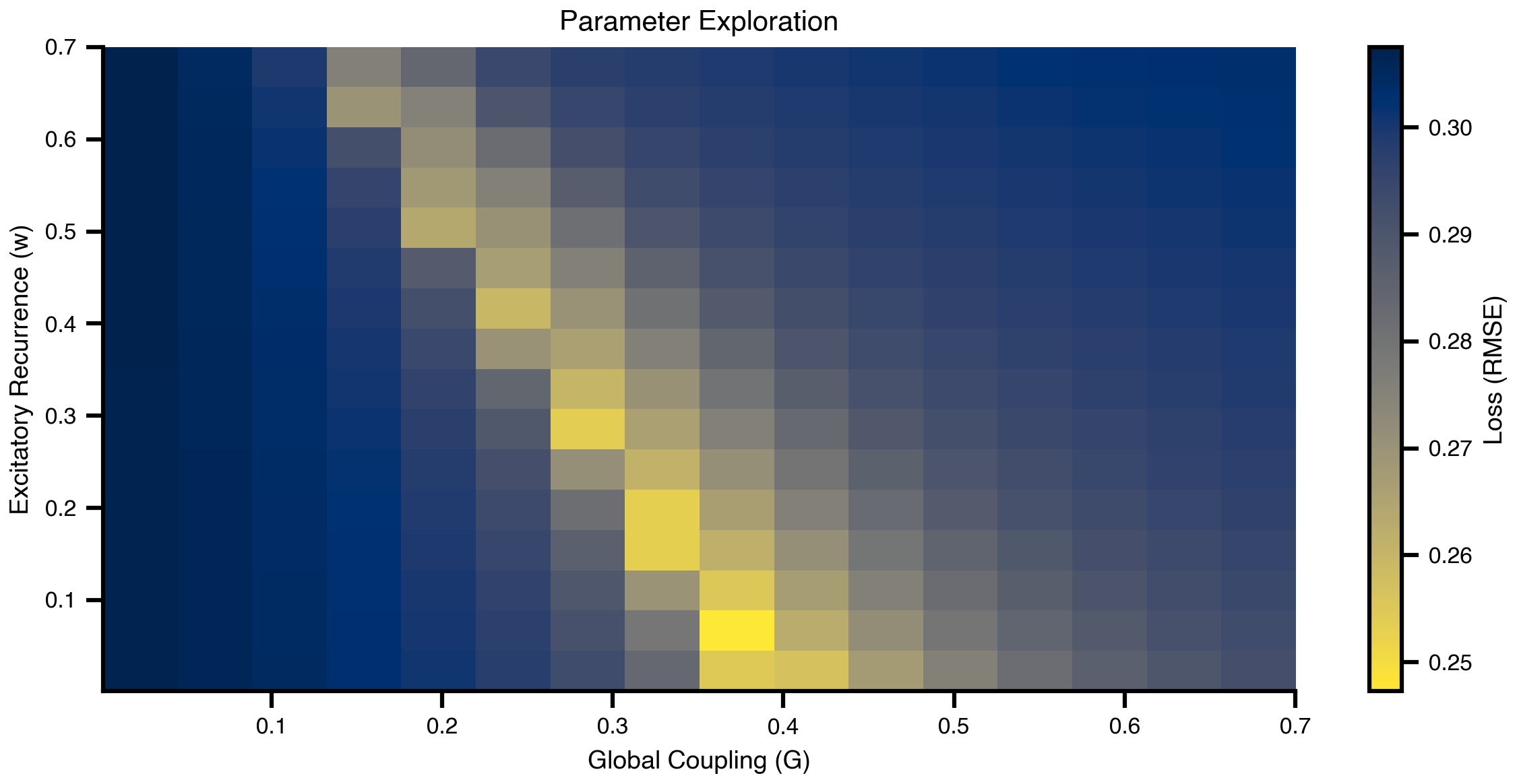
Before optimization, we explore how the model parameters affect FC quality. We systematically vary the excitatory recurrence w and global coupling strength G across a 2D grid and compute the loss for each combination.
New TVB-Optim concepts introduced here: GridAxis (a sweep range), Space (a collection of states to evaluate), ParallelExecution (runs the loss over the space), and @cache (skip the rerun if results already exist on disk).
# Create grid for parameter explorationn =16# Replace scalar values with GridAxis(...) to mark them as sweep axes:# each axis defines `n` linearly spaced values to try.grid_state = copy.deepcopy(state)grid_state.dynamics.w = GridAxis(0.001, 0.7, n)grid_state.coupling.instant.G = GridAxis(0.001, 0.7, n)# Space wraps the state into an iterable of all parameter combinations.# mode="product" -> Cartesian product (n*n = 256 evaluations);# mode="zip" would pair axes element-wise instead (n evaluations).grid = Space(grid_state, mode="product")# @cache stores the function's return value on disk under the given key.# On rerun, the cached result is loaded instead of recomputing. Set redo=True # to force recomputation if you change anything upstream (e.g. the loss).@cache("explore", redo=False)def explore():# n_pmap=8 maps evaluations across 8 JAX devices in parallel — this matches# the XLA_FLAGS device count set at the top of the notebook.exec= ParallelExecution(loss, grid, n_pmap=8)# Alternative: Sequential execution (RAM friendlier)# exec = SequentialExecution(loss, grid)returnexec.run()exploration_results = explore()
Figure 4: Parameter landscape exploration. The heatmap shows FC fitting loss (RMSE) across the parameter space of excitatory recurrence (w) and global coupling (G). Dark regions indicate better FC fits. The landscape reveals an optimal region where both parameters balance to reproduce empirical connectivity patterns.
9 Gradient-Based Optimization
We use gradient-based optimization to find the best global parameters (same values for all regions) that minimize the FC mismatch. JAX’s automatic differentiation computes gradients through the entire simulation pipeline.
New TVB-Optim concept: Parameter(...) is the wrapper that flips a value from “fixed constant” to “optimize me”. Anything not wrapped stays frozen.
# Wrap values in Parameter(...) to mark them as optimizable. The optimizer# walks the state tree, finds every Parameter, computes gradients w.r.t. the# loss, and updates them in place. Values left as plain floats stay fixed.state.coupling.instant.G = Parameter(state.coupling.instant.G)state.dynamics.w = Parameter(state.dynamics.w)# Create and run optimizercb = MultiCallback([ DefaultPrintCallback(every=10), SavingCallback(key="state", save_fun=lambda*args: args[1]) # Save updated state on every iteration for visualization])@cache("optimize", redo=False)def optimize(): opt = OptaxOptimizer(loss, optax.adam(0.01), callback=cb) fitted_state, fitting_data = opt.run(state, max_steps=100)return fitted_state, fitting_datafitted_state, fitting_data = optimize()
Figure 5: Optimization trajectory in parameter space. White points show the path taken by gradient descent from initial parameters (top marker) to optimized values (bottom marker). The optimizer efficiently navigates the loss landscape to find parameter combinations that yield good FC fits.
10 Heterogeneous Optimization
Global parameters (same for all regions) may not capture region-specific variations needed for optimal FC fit. We now make parameters heterogeneous: each brain region gets its own w value, while keeping G global.
New TVB-Optim concept: setting .shape on a Parameter broadcasts its current scalar value into a per-region array. The optimizer then treats each entry as an independent variable, going from 1 free parameter to n_nodes (here 84).
# Copy the already-optimized state so the heterogeneous fit starts from# the global optimum rather than from scratch.fitted_state_het = copy.deepcopy(fitted_state)# .shape = (n_nodes,) promotes the scalar w into a length-n_nodes vector,# initialized by broadcasting the current value. Each region then gets its# own gradient and is updated independently.fitted_state_het.dynamics.w.shape = (n_nodes,)# Unwrap G back to a plain value (Parameter -> .value) to freeze it during# this fit. Only Parameter-wrapped fields get optimized.fitted_state_het.coupling.instant.G = fitted_state_het.coupling.instant.G.valueshow_parameters(fitted_state_het)
Let’s compare the FC quality from global (homogeneous) vs regional (heterogeneous) parameter fits.
# Compute FC for both optimization strategiesfc_global = np.array(observation(fitted_state))fc_regional = np.array(observation(fitted_state_het))
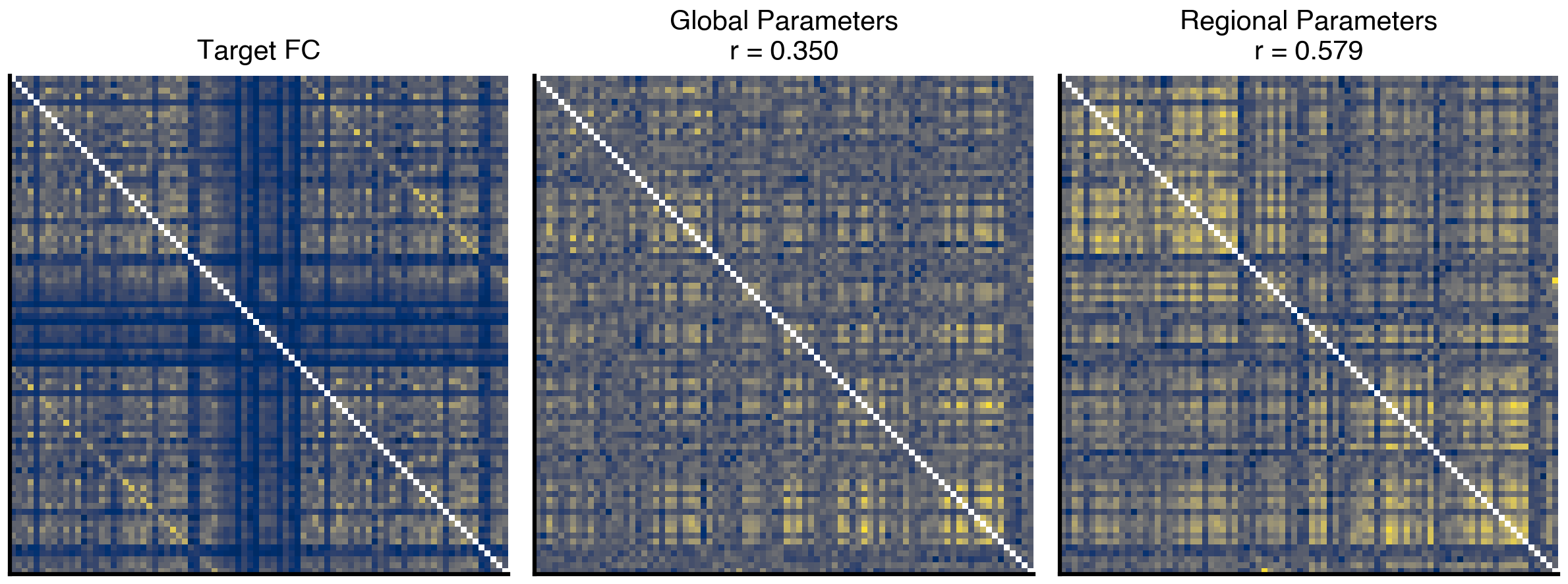
Figure 6: Comparison of functional connectivity matrices. Left: Empirical target FC from resting-state fMRI. Middle: FC from global parameter optimization. Right: FC from regional parameter optimization. The correlation coefficient (r) quantifies the similarity to the target FC. Regional parameters achieve better fit by accounting for local variations.
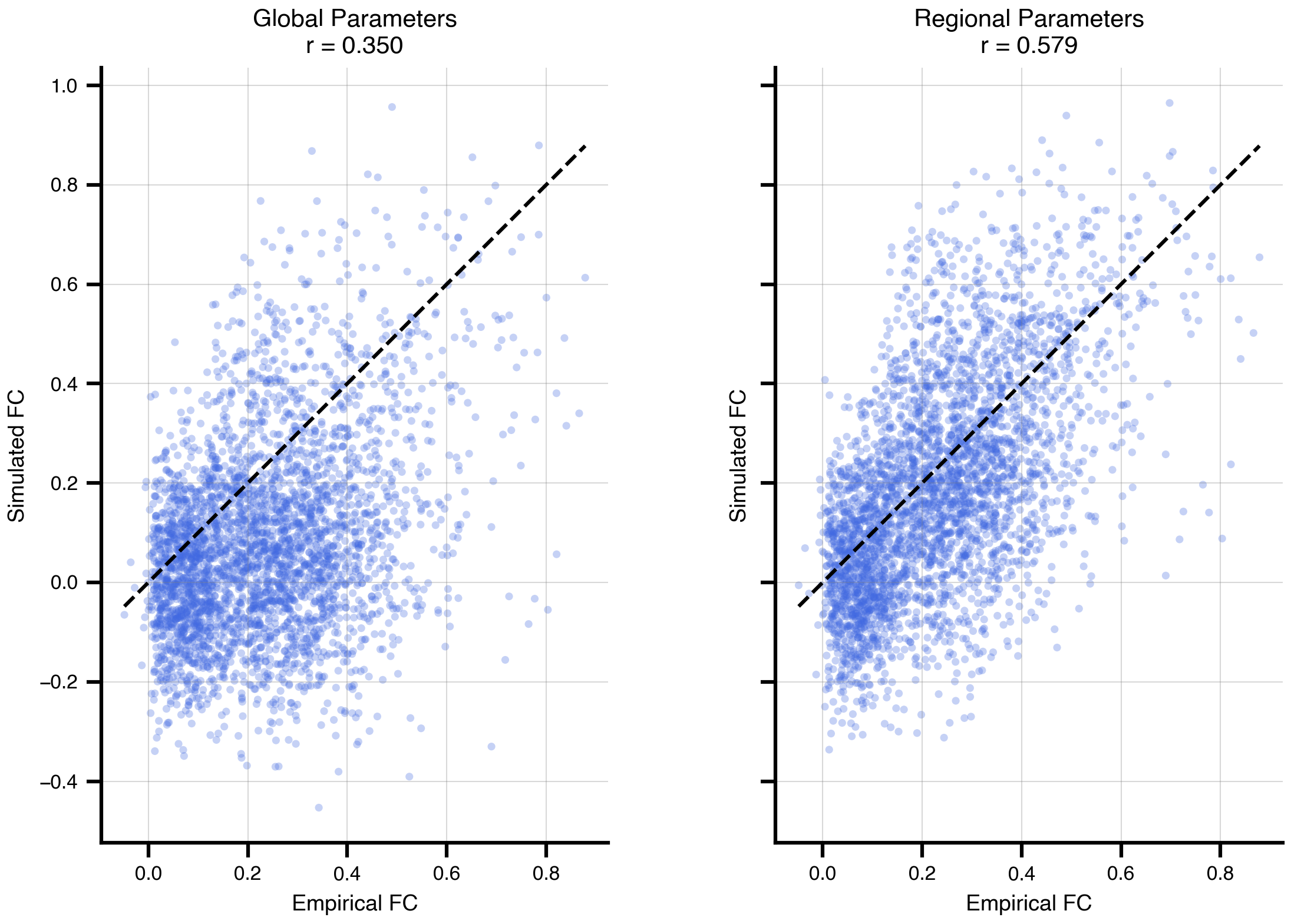
Figure 7: Scatter plots comparing fitted vs empirical FC. Each point represents one pairwise connection between brain regions. Left: Global parameter fit shows good overall correlation. Right: Regional parameter fit shows improved correlation with reduced scatter, indicating better reproduction of the empirical FC structure. The diagonal line represents perfect agreement.
12 Fitted Heterogeneous Parameters
Let’s examine the fitted region-specific parameters and their relationship to structural connectivity.
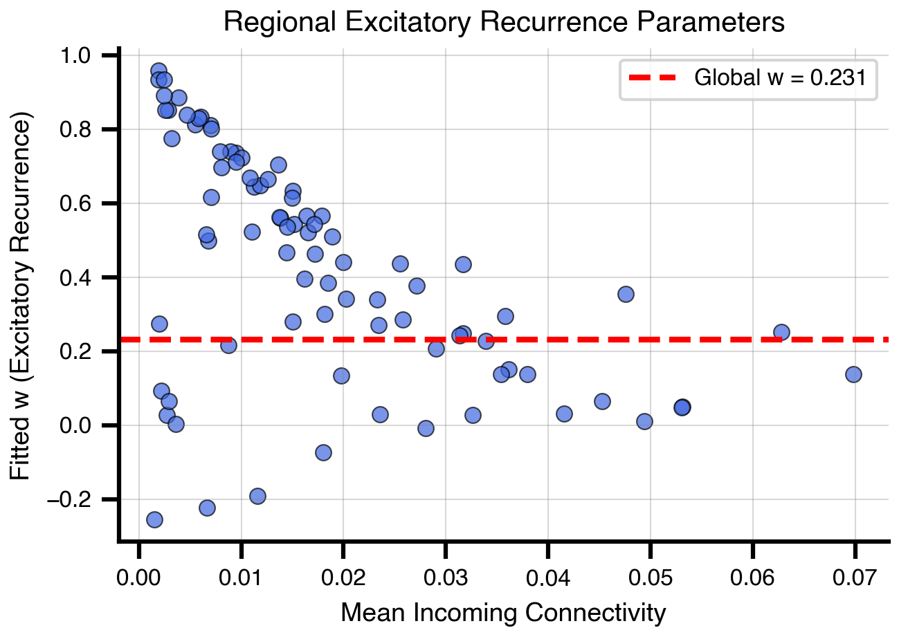
Figure 8: Fitted heterogeneous parameters. Fitted excitatory recurrence (w) for each region plotted against mean incoming structural connectivity strength. The dashed line shows the global optimization value for reference. Regions with stronger structural connections tend to require different parameter values to achieve optimal FC fit, demonstrating the importance of region-specific tuning.
Parameter Constraints
Notice that some regions have negative w values, which changes the biological interpretation of the parameter from excitatory to inhibitory recurrence. While this may be mathematically valid for achieving good FC fits, it violates the intended model constraints where w represents excitatory feedback strength.
In a further refinement step, we could use BoundedParameter to enforce physiological constraints during optimization:
# Example of using bounded parameters (not executed here)from tvboptim.types import BoundedParameter# Constrain w to positive values onlystate.dynamics.w = BoundedParameter( state.dynamics.w, lower_bound=0.0, # Enforce excitatory nature upper_bound=1.0# Maximum recurrence strength)
This would ensure that the optimizer only explores biologically plausible parameter regions while still allowing heterogeneous regional variations.
13 Exercises & Exploration
Disable 64-bit mode in JAX (restart the kernel). Rerun the fit, does it still work?
Explore different parameters (eg. dynamics.I_o, noise.sigma), add them to the optimization. Does that imporve the fit?
Try different optimizers (eg. optax.adamaxw vs optax.sgd), does it make a difference? You can also experiment with the learning rate.
Try optimizing with a shorter simulation length, it is faster but at which cost? Does a longer simulation improve the fit?
Switch to the 2 population Wong-Wang model (WongWangExcInh, w -> w_p), does it change the fit?