Installation & Requirements

TVBOptim requires Python 3.9 or later and depends on JAX for high-performance computing and automatic differentiation.

  1. Install the TVBO dependency

    This repository needs to be installed first. TVBO provides the brain simulation models, connectivity data and much more:

    git clone git@github.com:virtual-twin/tvbo.git
    cd tvbo
    pip install -e .
  2. Install TVBOptim

    TVBOptim provides utilities for optimization algorithms, parameter spaces, and execution strategies for TVBO models:

    git clone git@github.com:virtual-twin/tvboptim.git
    cd tvboptim
    pip install -e .

Create a TVBO Simulation Experiment

For all the details on TVBO, see its Documentation. A simple experiment can be created like this:

Imports
# Set up environment
import os
import time

# Mock devices to force JAX to parallelize on CPU (pmap trick)
# This allows parallel execution even without multiple GPUs
cpu = True
if cpu:
    N = 8  # Number of virtual devices to create
    os.environ['XLA_FLAGS'] = f'--xla_force_host_platform_device_count={N}'

# Import all required libraries
from scipy import io
import numpy as np
import matplotlib.pyplot as plt
import jax
import jax.numpy as jnp
import copy
import optax  # JAX-based optimization library
from IPython.display import Markdown

# Import from tvboptim - our optimization and execution framework
from tvboptim import jaxify  # Converts TVBO experiments to JAX functions
from tvboptim.types import Parameter, GridSpace  # Parameter types and spaces
from tvboptim.types.stateutils import show_free_parameters  # Utility functions
from tvboptim.utils import set_cache_path, cache  # Caching for expensive computations
from tvboptim import observation as obs  # Observation functions (FC, RMSE, etc.)
from tvboptim.execution import ParallelExecution, SequentialExecution  # Execution strategies
from tvboptim.optim.optax import OptaxOptimizer  # JAX-based optimizer with automatic differentiation
from tvboptim.optim.callbacks import MultiCallback, DefaultPrintCallback, SavingCallback  # Optimization callbacks

# Import from tvbo - the brain simulation framework
from tvbo.export.experiment import SimulationExperiment  # Main experiment class
from tvbo.datamodel import tvbo_datamodel  # Data structures
from tvbo.utils import numbered_print  # Utility functions

# Set cache path for tvboptim - stores expensive computations for reuse
set_cache_path("./example_cache_get_started")
# Create a brain simulation experiment using the Reduced Wong-Wang model
# This is a simplified neural mass model that captures excitatory dynamics
experiment = SimulationExperiment(
    model = {
        "name": "ReducedWongWang",  # Simplified version of Wong-Wang model
        "parameters": {
            "w": {"name": "w", "value": 0.5},      # Excitatory recurrence strength
            "I_o": {"name": "I_o", "value": 0.32}, # External input current
        },
        "state_variables": {
            "S": {"initial_value": 0.3},  # Set initial condition
        }
    },
    connectivity = {
        "parcellation": {"atlas": {"name": "DesikanKilliany"}},  # 87-region brain atlas
        "conduction_speed": {"name": "cs", "value": np.array([np.inf])}  # Infinite speed = no delays
    },
    coupling = {
        "name": "Linear",  # Linear coupling between brain regions
        "parameters": {"a": {"name": "a", "value": 0.75}}  # Global coupling strength
    },
    integration={
        "method": "Heun",      # Stochastic integration method
        "step_size": 4.0,      # Integration step size in ms
        "noise": {"parameters": {"sigma": {'value': 0.00283}}},  # Noise level
        "duration": 10_000     # Simulation duration in ms (10 seconds)
    },
    monitors={
        "Raw": {"name": "Raw"},  # Raw neural activity
        "Bold": {"name": "Bold", "period": 1000.0}},  # BOLD signal sampled every 1000ms
)

# Normalize connectivity weights to prevent runaway dynamics
experiment.connectivity.normalize_weights()
Markdown(experiment.model.generate_report())

ReducedWongWang

Reduced WongWang (RWW) is a biologically-inspired one-dimensional (i.e., only one state-variable ‘S’) neural mass model that approximates the realistic temporal dynamics of a detailed spiking and conductance-based synaptic large-scale network (Deco et al., 2013).

RWW is the dynamical mean-field (DMF) reduction of the Reduced WongWang Exc-Inh model, that consists in disentangling the contribution of the two neuronal populations (excitatory and inhibitory) in order to study the time evolution of just one pool of neurons for each network node (Wong & Wang, 2006). It results that the dynamics of each network node described the temporal evolution of the opening probability of the NMDA channels.

Equations

Derived Variables

\[ x = I_{o} + J_{N}*c_{global} + J_{N}*S*c_{local} + J_{N}*S*w \] \[ H = \frac{- b + a*x}{1 - e^{- d*\left(- b + a*x\right)}} \]

State Equations

\[ \frac{d}{d t} S = - \frac{S}{\tau_{s}} + H*\gamma*\left(1 - S\right) \]

Parameters

Parameter Value Unit Description
\(w\) 0.5 dimensionless Excitatory recurrence
\(I_{o}\) 0.32 nA External input current to the neurons population (Deco et al
\(J_{N}\) 0.2609 nA Excitatory recurrence
\(a\) 0.27 (pC)^-1 Slope (or gain) parameter of the sigmoid input-output function H_RWW (Deco et al
\(b\) 0.108 kHz Shift parameter of the sigmoid input-output function H_RWW (Deco et al
\(d\) 154.0 ms Scaling parameter of the sigmoid input-output function H_RWW (Deco et al
\(\gamma\) 0.641 N/A Kinetic parameter
\(\tau_{s}\) 100.0 ms Kinetic parameter

References

Citation key ‘Deco2013’ not found.

Citation key ‘WongWang2006’ not found.

numbered_print(experiment.render_code(format = "jax", scalar_pre = True))
001 
002 import jax.scipy.signal as sig
003 from collections import namedtuple
004 import jax
005 from tvbo.data.types import TimeSeries
006 import jax.numpy as jnp
007 import jax.scipy as jsp
008 
009 
010 def cfun(weights, history, current_state, p, delay_indices, t):
011     n_node = weights.shape[0]
012     a, b = p.a, p.b
013 
014     x_j = jnp.array([
015 
016         current_state[0],
017 
018     ])
019 
020     pre = x_j
021 
022     def op(x): return weights @ x
023     gx = jax.vmap(op, in_axes=0)(pre)
024     return b + a*gx
025 
026 
027 def dfun(current_state, cX, _p, local_coupling=0):
028     w, I_o, J_N, a, b, d, gamma, tau_s = _p.w, _p.I_o, _p.J_N, _p.a, _p.b, _p.d, _p.gamma, _p.tau_s
029     # unpack coupling terms and states as in dfun
030     c_pop0 = cX[0]
031 
032     S = current_state[0]
033 
034     # compute internal states for dfun
035     x = I_o + J_N*c_pop0 + J_N*S*local_coupling + J_N*S*w
036     H = (-b + a*x)/(1 - jnp.exp(-d*(-b + a*x)))
037 
038     return jnp.array([
039         -S/tau_s + H*gamma*(1 - S),  # S
040     ])
041 
042 
043 def integrate(state, weights, dt, params_integrate, delay_indices, external_input):
044     """
045     Heun Integration
046     ================
047     """
048     t, noise = external_input
049 
050     params_dfun, params_cfun, params_stimulus = params_integrate
051 
052     history, current_state = state
053     stimulus = 0
054 
055     inf = jnp.inf
056     min_bounds = jnp.array([[[0.0]]])
057     max_bounds = jnp.array([[[1.0]]])
058 
059     cX = jax.vmap(cfun, in_axes=(None, -1, -1, None, None, None), out_axes=-
060                   1)(weights, history, current_state, params_cfun, delay_indices, t)
061 
062     dX0 = dfun(current_state, cX, params_dfun)
063 
064     X = current_state
065 
066     # Calculate intermediate step X1
067     X1 = X + dX0 * dt + noise + stimulus * dt
068     X1 = jnp.clip(X1, min_bounds, max_bounds)
069 
070     # Calculate derivative X1
071     dX1 = dfun(X1, cX, params_dfun)
072     # Calculate the state change dX
073     dX = (dX0 + dX1) * (dt / 2)
074     next_state = current_state + (dX) + noise
075     next_state = jnp.clip(next_state, min_bounds, max_bounds)
076 
077     return (history, next_state), next_state
078 
079 
080 timeseries = namedtuple("timeseries", ["time", "trace"])
081 
082 
083 def monitor_raw_0(time_steps, trace, params, t_offset=0):
084     dt = 4.0
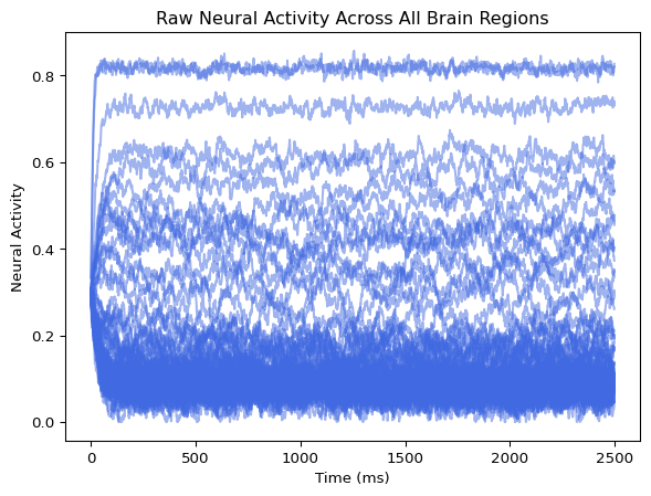
085     return TimeSeries(time=(time_steps + t_offset) * dt, data=trace, title="Raw")
086 
087 
088 def monitor_temporal_average_1(time_steps, trace, params, t_offset=0):
089     dt = 4.0
090     voi = jnp.array([0])
091     istep = 1
092     t_map = time_steps[::istep] - 1
093 
094     def op(ts):
095         start_indices = (ts,) + (0,) * (trace.ndim - 1)
096         slice_sizes = (istep,) + voi.shape + trace.shape[2:]
097         return jnp.mean(jax.lax.dynamic_slice(trace[:, voi, :], start_indices, slice_sizes), axis=0)
098     vmap_op = jax.vmap(op)
099     trace_out = vmap_op(t_map)
100 
101     idxs = jnp.arange(((istep - 2) // 2), time_steps.shape[0], istep)
102     return TimeSeries(time=(time_steps[idxs]) * dt, data=trace_out[0:idxs.shape[0], :, :], title="TemporalAverage")
103 
104 
105 exp, sin, sqrt = jnp.exp, jnp.sin, jnp.sqrt
106 
107 
108 def monitor_bold_1(time_steps, trace, params, t_offset=0):
109     # downsampling via temporal average / subsample
110     dt = 4.0
111     voi = jnp.array([0])
112     period = 1000.0  # sampling period of the BOLD Monitor in ms
113     istep_int = 1  # steps taken by the averaging/subsampling monitor to get an interim period of 4 ms
114     istep = 250
115     final_istep = 250  # steps to take on the downsampled signal
116 
117     res = monitor_temporal_average_1(time_steps, trace, None)
118     time_steps_i = res.time
119     trace_new = res.data
120 
121     time_steps_new = time_steps[jnp.arange(
122         istep-1, time_steps.shape[0], istep)]
123 
124     # hemodynamic response function
125     tau_s = params.tau_s
126     tau_f = params.tau_f
127     k_1 = params.k_1
128     V_0 = params.V_0
129     stock = params.stock
130 
131     trace_new = jnp.vstack([stock, trace_new])
132 
133     def op(var): return 1/3. * exp(-0.5*(var / tau_s)) * (sin(sqrt(1. /
134                                                                    tau_f - 1./(4.*tau_s**2)) * var)) / (sqrt(1./tau_f - 1./(4.*tau_s**2)))
135     stock_steps = 5000
136     stock_time_max = 20.0  # stock time has to be in seconds
137     stock_time_step = stock_time_max / stock_steps
138     stock_time = jnp.arange(0.0, stock_time_max, stock_time_step)
139     hrf = op(stock_time)
140 
141     # Convolution along time axis
142     # via fft
143     def op1(x): return sig.fftconvolve(x, hrf, mode="valid")
144 
145     def op2(x): return jax.vmap(op1, in_axes=(
146         1), out_axes=(1))(x)  # map over nodes
147     def op3(x): return jax.vmap(op2, in_axes=(1), out_axes=(1))(
148         x)  # map over state variables
149     bold = jax.vmap(op3, in_axes=(3), out_axes=(3))(
150         trace_new)  # map over modes
151 
152     bold = k_1 * V_0 * (bold - 1.0)
153 
154     bold_idx = jnp.arange(
155         final_istep-2, time_steps_i.shape[0], final_istep)[0:time_steps_new.shape[0]] + 1
156     return TimeSeries(time=(time_steps_new + t_offset) * dt, data=bold[bold_idx, :, :], title="BOLD")
157 
158 
159 def transform_parameters(_p):
160     w, I_o, J_N, a, b, d, gamma, tau_s = _p.w, _p.I_o, _p.J_N, _p.a, _p.b, _p.d, _p.gamma, _p.tau_s
161 
162     return _p
163 
164 
165 c_vars = jnp.array([0])
166 
167 
168 def kernel(state):
169     # problem dimensions
170     n_nodes = 87
171     n_svar = 1
172     n_cvar = 1
173     n_modes = 1
174     nh = 1
175 
176     # history = current_state
177     current_state, history = (state.initial_conditions.data[-1], None)
178 
179     ics = (history, current_state)
180     weights = state.connectivity.weights
181 
182     dn = jnp.arange(n_nodes) * jnp.ones((n_nodes, n_nodes)).astype(int)
183     idelays = jnp.round(state.connectivity.lengths /
184                         state.connectivity.metadata.conduction_speed.value / state.dt).astype(int)
185     di = -1 * idelays - 1
186     delay_indices = (di, dn)
187 
188     dt = state.dt
189     nt = state.nt
190     time_steps = jnp.arange(0, nt)
191 
192     key = jax.random.PRNGKey(state.noise.metadata.seed)
193     _noise = jax.random.normal(key, (nt, n_svar, n_nodes, n_modes))
194     noise = (jnp.sqrt(dt) * state.noise.sigma[None, ..., None, None]) * _noise
195 
196     p = transform_parameters(state.parameters.model)
197     params_integrate = (p, state.parameters.coupling, state.stimulus)
198 
199     def op(ics, external_input): return integrate(ics, weights,
200                                                   dt, params_integrate, delay_indices, external_input)
201 
202     latest_carry, res = jax.lax.scan(op, ics, (time_steps, noise))
203 
204     trace = res
205 
206     t_offset = 0
207     time_steps = time_steps + 1
208 
209     params_monitors = state.monitor_parameters
210     result = [monitor_raw_0(time_steps, trace, params_monitors[0], t_offset=t_offset),
211               monitor_bold_1(time_steps, trace,
212                              params_monitors[1], t_offset=t_offset),
213               ]
214 
215     return result

Get Model and State

The jaxify function converts the TVBO experiment into a JAX-compatible model function and state object. The scalar_pre option is used to improve performance when we have no delay (infinite conduction speed):

# Convert TVBO experiment to JAX function and state
# scalar_pre=True optimizes for no-delay scenarios
model, state = jaxify(experiment, scalar_pre = True)

The model is now a JAX-compiled function that can be called with a state to run the simulation. The state contains all parameters, initial conditions, and configuration needed for the simulation.

Understand the State Object & Parameters

The state is of type tvbo.datamodel.tvbo_datamodel.Bunch, which is a dict with convenient get and set functions. At the same time, it is also a jax.Pytree, making it compatible with all of JAX’s transformations. You can think of it as a big tree holding all parameters and initial conditions that uniquely define a simulation:

state
SimulationState
├── initial_conditions
│   ├── time
│   │   ├── _name: ""
│   │   ├── _value: f64[1]
│   │   ├── _free: False
│   │   ├── low: NoneType
│   │   ├── high: NoneType
│   │   └── doc: NoneType
│   ├── data
│   │   ├── _name: ""
│   │   ├── _value: f64[1,1,87,1]
│   │   ├── _free: False
│   │   ├── low: NoneType
│   │   ├── high: NoneType
│   │   └── doc: NoneType
│   ├── labels_dimensions
│   │   ├── [0]: "Time"
│   │   ├── [1]: "State Variable"
│   │   ├── [2]: "Space"
│   │   └── [3]: "Mode"
│   ├── title: "TimeSeries"
│   ├── connectivity: NoneType
│   ├── sample_period: NoneType
│   ├── dt: NoneType
│   ├── sample_period_unit: "ms"
│   └── labels_ordering
│       ├── [0]: "Time"
│       ├── [1]: "State Variable"
│       ├── [2]: "Space"
│       └── [3]: "Mode"
├── connectivity
│   ├── weights
│   │   ├── _name: ""
│   │   ├── _value: f64[87,87]
│   │   ├── _free: False
│   │   ├── low: NoneType
│   │   ├── high: NoneType
│   │   └── doc: NoneType
│   ├── lengths: f64[87,87](numpy)
│   └── metadata: Connectome
├── dt
│   ├── _name: ""
│   ├── _value: f64[]
│   ├── _free: False
│   ├── low: NoneType
│   ├── high: NoneType
│   └── doc: NoneType
├── noise
│   ├── sigma
│   │   ├── _name: ""
│   │   ├── _value: f64[]
│   │   ├── _free: False
│   │   ├── low: NoneType
│   │   ├── high: NoneType
│   │   └── doc: NoneType
│   ├── nsig
│   │   ├── _name: ""
│   │   ├── _value: f64[]
│   │   ├── _free: False
│   │   ├── low: NoneType
│   │   ├── high: NoneType
│   │   └── doc: NoneType
│   └── metadata: Noise
├── parameters
│   ├── model
│   │   ├── w
│   │   │   ├── _name: ""
│   │   │   ├── _value: f64[]
│   │   │   ├── _free: False
│   │   │   ├── low: NoneType
│   │   │   ├── high: NoneType
│   │   │   └── doc: NoneType
│   │   ├── I_o
│   │   │   ├── _name: ""
│   │   │   ├── _value: f64[]
│   │   │   ├── _free: False
│   │   │   ├── low: NoneType
│   │   │   ├── high: NoneType
│   │   │   └── doc: NoneType
│   │   ├── J_N
│   │   │   ├── _name: ""
│   │   │   ├── _value: f64[]
│   │   │   ├── _free: False
│   │   │   ├── low: NoneType
│   │   │   ├── high: NoneType
│   │   │   └── doc: NoneType
│   │   ├── a
│   │   │   ├── _name: ""
│   │   │   ├── _value: f64[]
│   │   │   ├── _free: False
│   │   │   ├── low: NoneType
│   │   │   ├── high: NoneType
│   │   │   └── doc: NoneType
│   │   ├── b
│   │   │   ├── _name: ""
│   │   │   ├── _value: f64[]
│   │   │   ├── _free: False
│   │   │   ├── low: NoneType
│   │   │   ├── high: NoneType
│   │   │   └── doc: NoneType
│   │   ├── d
│   │   │   ├── _name: ""
│   │   │   ├── _value: f64[]
│   │   │   ├── _free: False
│   │   │   ├── low: NoneType
│   │   │   ├── high: NoneType
│   │   │   └── doc: NoneType
│   │   ├── gamma
│   │   │   ├── _name: ""
│   │   │   ├── _value: f64[]
│   │   │   ├── _free: False
│   │   │   ├── low: NoneType
│   │   │   ├── high: NoneType
│   │   │   └── doc: NoneType
│   │   └── tau_s
│   │       ├── _name: ""
│   │       ├── _value: f64[]
│   │       ├── _free: False
│   │       ├── low: NoneType
│   │       ├── high: NoneType
│   │       └── doc: NoneType
│   ├── integration
│   │   └── noise
│   │       └── sigma
│   │           ├── _name: ""
│   │           ├── _value: f64[]
│   │           ├── _free: False
│   │           ├── low: NoneType
│   │           ├── high: NoneType
│   │           └── doc: NoneType
│   └── coupling
│       ├── a
│       │   ├── _name: ""
│       │   ├── _value: f64[]
│       │   ├── _free: False
│       │   ├── low: NoneType
│       │   ├── high: NoneType
│       │   └── doc: NoneType
│       └── b
│           ├── _name: ""
│           ├── _value: f64[]
│           ├── _free: False
│           ├── low: NoneType
│           ├── high: NoneType
│           └── doc: NoneType
├── stimulus: NoneType
├── monitor_parameters
│   ├── 0: Bunch
│   └── 1
│       ├── tau_s
│       │   ├── _name: ""
│       │   ├── _value: f64[]
│       │   ├── _free: False
│       │   ├── low: NoneType
│       │   ├── high: NoneType
│       │   └── doc: NoneType
│       ├── tau_f
│       │   ├── _name: ""
│       │   ├── _value: f64[]
│       │   ├── _free: False
│       │   ├── low: NoneType
│       │   ├── high: NoneType
│       │   └── doc: NoneType
│       ├── k_1
│       │   ├── _name: ""
│       │   ├── _value: f64[]
│       │   ├── _free: False
│       │   ├── low: NoneType
│       │   ├── high: NoneType
│       │   └── doc: NoneType
│       ├── V_0
│       │   ├── _name: ""
│       │   ├── _value: f64[]
│       │   ├── _free: False
│       │   ├── low: NoneType
│       │   ├── high: NoneType
│       │   └── doc: NoneType
│       └── stock
│           ├── _name: ""
│           ├── _value: f64[5000,1,87,1]
│           ├── _free: False
│           ├── low: NoneType
│           ├── high: NoneType
│           └── doc: NoneType
└── nt: 2500

Each leaf of the tree (in JAX, that is each JAX Array) is wrapped in the Parameter type. This enables additional convenience functionality. A Parameter can be declared free, making it available to Spaces or to gradients during optimization.

# Mark the excitatory recurrence parameter as free for optimization
state.parameters.model.J_N.free = True
show_free_parameters(state)  # Display all parameters marked as free
FreeState
├── initial_conditions: TimeSeries
├── connectivity: Connectome
├── noise: Noise
├── parameters
│   ├── model
│   │   ├── J_N
│   │   │   ├── _name: ""
│   │   │   ├── _value: 0.2609
│   │   │   ├── _free: True
│   ├── integration: Bunch
│   └── coupling: Bunch
├── monitor_parameters: dict
└── nt: 2500

If your simulation needs additional Parameters or data, you can simply put a new leaf into the state:

# Example: Add a custom optimizable parameter to the state
# This demonstrates how to extend the state with additional parameters
state.parameters.important_extras = Parameter("Important", jnp.zeros(10), free = True)
show_free_parameters(state)  # Now shows both J_N and our custom parameter
FreeState
├── initial_conditions: TimeSeries
├── connectivity: Connectome
├── noise: Noise
├── parameters
│   ├── model
│   │   ├── J_N
│   │   │   ├── _name: ""
│   │   │   ├── _value: 0.2609
│   │   │   ├── _free: True
│   ├── integration: Bunch
│   ├── coupling: Bunch
│   └── important_extras
│       ├── _name: "Important"
│       ├── _value: [0. 0. 0. 0. 0. 0. 0. 0. 0. 0.]
│       ├── _free: True
├── monitor_parameters: dict
└── nt: 2500

Simulate the Model

To run a simulation, you can simply call the model.

# Run the simulation - model returns (raw_activity, bold_signal)
result = model(state)
raw, bold = result

# Plot raw neural activity for all 87 brain regions over time
# Shape: [time_points, state_variables, regions, modes]
plt.plot(raw.data[:,0,:,0], color = "royalblue", alpha = 0.5)
plt.xlabel("Time (ms)")
plt.ylabel("Neural Activity")
plt.title("Raw Neural Activity Across All Brain Regions");

Wrap the Model to create observations

We look at the mean activity of the last 500 timesteps as an easy observation.

def observation(state):
    """
    Extract a simple observation from the simulation.
    We use the mean activity of the last 500 timesteps to avoid transient effects.
    """
    ts = model(state)[0].data[-500:,0,:,0]  # Last 500 timesteps, skip transient
    mean_activity = jnp.mean(ts)  # Average across time and regions
    return mean_activity

# Test the observation function
print(f"Mean activity: {observation(state):.4f}")
Mean activity: 0.1752

Explore that across a parameter space

We can use a GridSpace to explore how parameters J_N (excitatory recurrence) and a (global coupling) affect the observation. We use the cache decorator to save computationally demanding operations. We also parallelize the exploration using the ParallelExecution class with n_pmap = 8, which is possible because we told JAX that our CPU has 8 devices - known as the pmap trick.

# Clean up: disable the custom parameter we added earlier
state.parameters.important_extras.free = False

# Set up parameter exploration for two key parameters
# a: global coupling strength
state.parameters.coupling.a.free = True
state.parameters.coupling.a.low = 0.0   # Lower bound
state.parameters.coupling.a.high = 1.0  # Upper bound

# J_N: NMDA synaptic coupling strength
state.parameters.model.J_N.free = True
state.parameters.model.J_N.low = 0.0
state.parameters.model.J_N.high = 1.0

# Create a grid space for systematic parameter exploration
n = 32  # 32x32 grid = 1024 parameter combinations
params_set = GridSpace(state, n=n)

@cache("explore", redo = False)  # Cache results to avoid recomputation
def explore():
    # Use parallel execution with 8 virtual devices (pmap trick)
    exec = ParallelExecution(observation, params_set, n_pmap=8)
    return exec.run()

# Run the exploration (or load from cache)
exploration = explore()

# Visualize the parameter space exploration
plt.figure(figsize=(8, 6))
plt.imshow(jnp.stack(exploration).reshape(n, n), aspect = "auto", extent=[0, 1, 0, 1])
plt.xlabel("a")
plt.ylabel("J_N")
plt.title("Mean Activity Across Parameter Space")
plt.colorbar(label="Mean Activity")
Loading explore from cache, last modified 2025-07-03 15:06:34.498307

Define a Loss and Optimize

Let’s say our goal is to have a mean activity of 0.5. We can define a loss function that penalizes deviations from this target.

def loss(state):
    """
    Define a loss function that penalizes deviations from target activity.
    Goal: Each brain region should have mean activity of 0.5
    """
    ts = model(state)[0].data[-500:,0,:,0]  # Skip transient period
    mean_activity = jnp.mean(ts, axis = 0)  # Average over time for each region
    # Compute mean squared error between actual and target (0.5) activity
    return jnp.mean((mean_activity - 0.5)**2)  # Region-wise difference

# Test the loss function
print(f"Current loss: {loss(state):.6f}")
Current loss: 0.135816

Then we optimize it with Optax and gradient descent:

# Create an optimizer using Adam with automatic differentiation
optimizer = OptaxOptimizer(
    loss,                           # Loss function to minimize
    optax.adam(0.005),             # Adam optimizer with learning rate 0.005
    callback=DefaultPrintCallback(every=5) # Print progress during optimization
)

# Run optimization using forward-mode automatic differentiation
# Forward mode is efficient when we have few parameters (like here: a and J_N)
optimized_state, _ = optimizer.run(state, max_steps=50, mode="fwd")
Step 0: 0.135816
Step 5: 0.107015
Step 10: 0.087062
Step 15: 0.077474
Step 20: 0.074584
Step 25: 0.073727
Step 30: 0.073262
Step 35: 0.073115
Step 40: 0.073099
Step 45: 0.073084

Visualize the Fitted Model

# Simulate with optimized parameters and visualize results
ts_optimized = model(optimized_state)[0].data[:,0,:,0]

plt.figure(figsize=(10, 6))
plt.plot(ts_optimized, alpha = 0.5, color = "royalblue")
plt.hlines(0.5, 0, 2500, color = "black", linewidth = 2.5, label="Target (0.5)")
plt.hlines(observation(optimized_state), 0, 2500, color = "red", linewidth = 2.5, 
           label=f"Actual Mean ({observation(optimized_state):.3f})")
plt.xlabel("Time (ms)")
plt.ylabel("Neural Activity")
plt.title("Optimized Neural Activity")
plt.legend()
plt.grid(True, alpha=0.3)

Well, the mean is close to the target, but most regions are either too high or too low. We can make parameters heterogeneous to adjust that.

Heterogeneous Parameters

The previous optimization used global parameters (same value for all brain regions). Now we’ll make parameters region-specific to achieve better control:

# Make parameters heterogeneous: one value per brain region (87 regions)
optimized_state.parameters.model.J_N.shape = (87,1)  # Excitatory recurrence per region
print(f"J_N parameter shape: {optimized_state.parameters.model.J_N.shape}")
J_N parameter shape: (87, 1)

We switch to reverse mode automatic differentiation, which is more efficient when we have many parameters (87 parameters):

# Create optimizer for heterogeneous parameters
optimizer_het = OptaxOptimizer(
    loss,                                    # Same loss function
    optax.adam(0.002),                      # Lower learning rate for stability
    callback=DefaultPrintCallback(every=10) # Print every 10 steps
)

# Use reverse-mode AD (more efficient for many parameters)
optimized_state_het, _ = optimizer_het.run(optimized_state, max_steps=200, mode="rev")
Step 0: 0.073036
Step 10: 0.061548
Step 20: 0.050403
Step 30: 0.041717
Step 40: 0.032587
Step 50: 0.024754
Step 60: 0.014539
Step 70: 0.006013
Step 80: 0.008035
Step 90: 0.005476
Step 100: 0.011970
Step 110: 0.013880
Step 120: 0.015561
Step 130: 0.013589
Step 140: 0.014465
Step 150: 0.014972
Step 160: 0.011115
Step 170: 0.013463
Step 180: 0.012640
Step 190: 0.011850

Now most regions are close to the target level after passing the initial transient. Setting the initial conditions to the target activity could be a solution to this problem.

# Visualize results with heterogeneous parameters
ts_optimized_het = model(optimized_state_het)[0].data[:,0,:,0]

plt.figure(figsize=(15, 10))

# Plot 1: Time series for all regions
plt.subplot(2, 1, 1)
plt.plot(ts_optimized_het, alpha = 0.5, color = "royalblue")
plt.hlines(0.5, 0, 2500, color = "black", linewidth = 2.5, label="Target (0.5)")
plt.hlines(observation(optimized_state_het), 0, 2500, color = "red", linewidth = 2.5, 
           label=f"Mean ({observation(optimized_state_het):.3f})")
plt.xlabel("Time (ms)")
plt.ylabel("Neural Activity")
plt.title("Heterogeneous Optimization")
plt.legend()
plt.grid(True, alpha=0.3)

# Plot 2: J_N parameters vs mean regionwise coupling
mean_coupling = jnp.mean(experiment.connectivity.weights, axis=1)
plt.subplot(2, 1, 2)
plt.scatter(mean_coupling, optimized_state_het.parameters.model.J_N.value.flatten(), alpha=0.7, color="k", s=30)
plt.xlabel("Mean Regionwise Coupling")
plt.ylabel("J_N [nA]")
plt.title("Fitted J_N Parameters")
plt.grid(True, alpha=0.3)
plt.legend()

plt.tight_layout()
/tmp/ipykernel_166174/1020819468.py:26: UserWarning:

No artists with labels found to put in legend.  Note that artists whose label start with an underscore are ignored when legend() is called with no argument.

Why is this problem interesting? The Reduced Wong Wang model has two fixed point branches - low activity (~0.1) and high activity (~0.9). Each region tends to approach one of them, but for the desired target level, we need to find a balance between the two. This concept is also known as feedback inhibition control (FIC).

Key Concepts Demonstrated

This tutorial showcased several important TVBOptim concepts:

  1. Parameter Types: The Parameter class wraps JAX arrays with additional metadata (bounds, free/fixed status)
  2. State Management: The state object is a JAX PyTree containing all simulation parameters and initial conditions
  3. Spaces: GridSpace and UniformSpace enable systematic parameter exploration
  4. Execution Strategies: ParallelExecution leverages JAX’s pmap for efficient computation across parameter sets
  5. Optimization: OptaxOptimizer provides gradient-based optimization with automatic differentiation
  6. Caching: The @cache decorator saves expensive computations for reuse
  7. Heterogeneous Parameters: Region-specific parameters enable fine-grained control over brain dynamics

These tools enable efficient exploration and optimization of complex brain network models at scale.