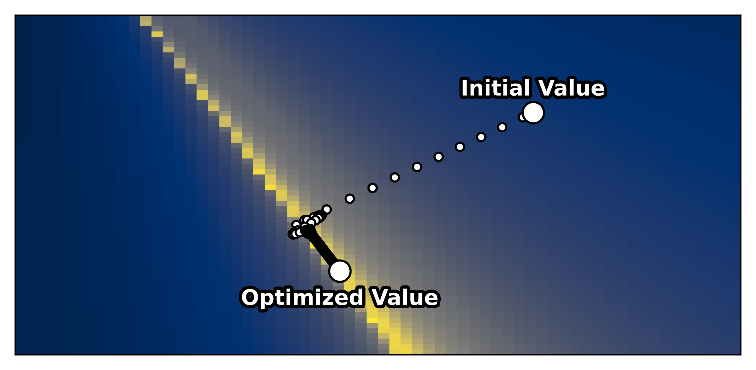
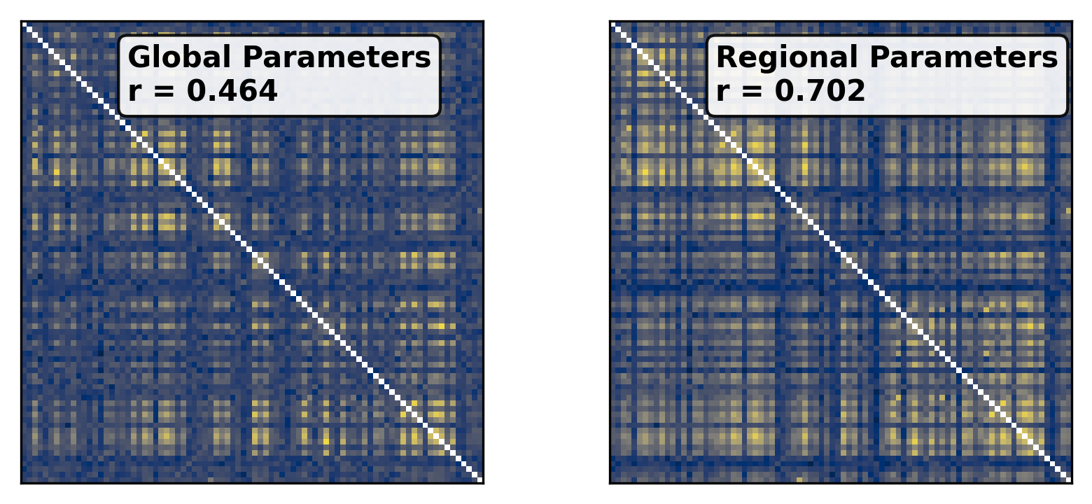
--- title: "Reduced Wong Wang BOLD FC Optimization" format: html: code-fold: false toc: true echo: false jupyter: python3 --- ```{python} #| output: false #| code-fold: true #| code-summary: "Imports" #| echo: true # Set up environment import osimport time# Mock devices to force JAX to parallelize on CPU = True if cpu:= 8 'XLA_FLAGS' ] = f'--xla_force_host_platform_device_count= { N} ' # Import all required libraries from scipy import ioimport numpy as npimport matplotlib.pyplot as pltimport jaximport jax.numpy as jnpimport copyimport optax# Import from tvboptim from tvboptim import jaxifyfrom tvboptim.types import Parameter, GridSpacefrom tvboptim.types.stateutils import show_free_parametersfrom tvboptim.utils import set_cache_path, cachefrom tvboptim import observation as obsfrom tvboptim.execution import ParallelExecution, SequentialExecutionfrom tvboptim.optim.optax import OptaxOptimizerfrom tvboptim.optim.callbacks import MultiCallback, DefaultPrintCallback, SavingCallback# Import from tvbo from tvbo.export.experiment import SimulationExperimentfrom tvbo.datamodel import tvbo_datamodelfrom tvbo.utils import numbered_print# Set cache path for tvboptim "./example_cache_rww" )``` ## Create a TVB-O Simulation Experiment ```{python} #| echo: true #| output: false = SimulationExperiment(= {"name" : "ReducedWongWang" , "parameters" : {"w" : {"name" : "w" , "value" : 0.5 },"I_o" : {"name" : "I_o" , "value" : 0.32 }, = {"parcellation" : {"atlas" : {"name" : "DesikanKilliany" }}, "conduction_speed" : {"name" : "cs" , "value" : np.array([np.inf])}= {"name" : "Linear" , "parameters" : {"a" : {"name" : "a" , "value" : 0.5 }}= {"method" : "Heun" ,"step_size" : 4.0 ,"noise" : {"parameters" : {"sigma" : {'value' : 0.00283 }}},"duration" : 2 * 60_000 = {"Raw" : {"name" : "Raw" }, "Bold" : {"name" : "Bold" , "period" : 1000.0 }},``` ```{python} = io.loadmat("../data/avgSC_DK.mat" ,= True ,= False ,= True ,= io.loadmat( "../data/avgFC_DK.mat" , squeeze_me= True , mat_dtype= False , chars_as_strings= True , )= fcdata["avgFC" ]= np.array(data["SC_avg_weights" ], dtype= np.float64)= np.array(data["SC_avg_dists" ], dtype= np.float64)= lengths= weights = weights.shape[1 ]# tvbo_datamodel.Connectome(weights = weights, lengths = lengths, conduction_speed = np.array([np.inf])) ``` ```{python} = plt.subplots(1 , 2 , figsize = (8 , 4 ), sharey= True )= ax1.imshow(experiment.connectivity.weights, cmap = "cividis" , vmax = .5 )"Structural Connectivity" )"Region" )"Region" )= fig.colorbar(im1, ax= ax1, shrink= 0.74 , label= "Connection Strength [a.u.]" , extend= 'max' )= ax2.imshow(experiment.connectivity.lengths, cmap = "cividis" )"Tract Lengths" )"Region" )= fig.colorbar(im2, ax= ax2, shrink= 0.74 , label= "Tract Length [mm]" )= 200 ``` ## Model Functions ```{python} # Get model and state - scalar_pre is used to improve performance as we have no delay #| echo: true = jaxify(experiment, scalar_pre = True )``` ## Rendered JAX Code ```{python} #| echo: true format = "jax" , scalar_pre = True ))``` ## Run Initial Simulation - Update Inital Conditions ```{python} #| echo: true # Run the model and get results = model(state)# Use first result as initial conditions for second run = result[0 ]# select last 5000 steps as BOLD stock 1 ]["stock" ] = result[0 ].data[- 5000 :]= model(state)``` ```{python} from matplotlib.colors import Normalize# Plot time series from both simulations = plt.subplots(1 , 2 , figsize= (6 , 2 ))= 1000 # For the first plot (Raw) = result2[0 ].time[0 :t_max]= result2[0 ].data[0 :t_max,0 ,:,0 ]# If data1 is multi-dimensional, we need to handle each line separately = data1.shape[1 ]# Create a colormap with distinct colors for each line based on its mean = plt.cm.cividis= np.mean(data1, axis= 0 ) # Mean for each line = Normalize(vmin= np.min (mean_values), vmax= np.max (mean_values))for i in range (num_lines):= cmap(norm(mean_values[i]))= color, linewidth= 0.5 )# Add title as text inside the plot 0.95 , 0.95 , "Raw" , transform= ax1.transAxes, fontsize= 12 , = 'right' , va= 'top' , bbox= dict (boxstyle= "round,pad=0.3" , facecolor= 'white' , alpha= 0.8 ))"Time [ms]" )"S [a.u.]" ) # Add y-label as requested # For the second plot (Bold) - similar approach = result2[1 ].time[0 :60 ]= result2[1 ].data[0 :60 ,0 ,:,0 ]# If data2 is multi-dimensional, handle each line separately = data2.shape[1 ]# Create a colormap with distinct colors for each line based on its mean # cmap = plt.cm.viridis = np.mean(data2, axis= 0 )= Normalize(vmin= np.min (mean_values), vmax= np.max (mean_values))for i in range (num_lines):= cmap(norm(mean_values[i]))= color, linewidth= 0.8 )# Add title as text inside the plot 0.95 , 0.95 , "Bold" , transform= ax2.transAxes, fontsize= 12 , = 'right' , va= 'top' , bbox= dict (boxstyle= "round,pad=0.3" , facecolor= 'white' , alpha= 0.8 ))"Time [ms]" )# ax2.set_ylabel("Value [a.u.]") # Add y-label as requested 500 )# plt.tight_layout() ``` ## Define Observations and Loss ```{python} #| echo: true def observation(state):= model(state)[1 ]return obs.fc(bold, skip_t = 20 )def loss(state):= observation(state)# return 1 - obs.fc_corr(fc, fc_target) return obs.rmse(fc, fc_target)``` ```{python} # Calculate the functional connectivity matrix = np.array(obs.fc(result2[1 ], skip_t = 20 ))# Create the figure and axis = plt.subplots(1 ,2 , figsize= (6 , 2 ))# Plot the FC matrix for ax_current, fc_matrix, title in zip ([ax2, ax], [fc_target, fc_], ["Target FC" , "Observed FC \n r = {:.3f} " .format (obs.fc_corr(fc_, fc_target))]):= np.copy(fc_matrix)# Set diagonal to NaN to handle them separately = ax_current.imshow(fc_matrix, cmap= 'cividis' , vmax = 0.9 )# Remove x-axis ticks # Remove y-axis ticks '' ) # Remove x-axis label '' )# Add title as annotation inside the plot = (0.3 , 0.95 ), # Position in axes coordinates = 'axes fraction' ,= 'left' , va= 'top' ,= 10 , fontweight= 'bold' ,= 'black' , # Black text on white background = dict (boxstyle= 'round,pad=0.3' , = 'white' , alpha= 0.9 ))# Add colorbar (uncomment if needed) # cbar = plt.colorbar(im, ax=ax) # cbar.set_label("Correlation") 300 )``` ```{python} #| output: false # import matplotlib.transforms as transforms# Calculate the functional connectivity matrix (keep this line as reference) # fc_ = np.array(fc(result2[1], skip_t = 20)) # Create the figure and axis = plt.subplots(figsize= (3 , 3 ))# Create a mask for the upper triangle = np.triu(np.ones_like(fc_target), k= 1 ).astype(bool )# Apply mask to the FC matrix (create a copy first) = np.copy(fc_target)= np.nan # Set upper triangle to NaN # Set diagonal to NaN import matplotlib.colors as mcolors= ['#9C27B0' , # Purple/Violet '#00BCD4' , # Cyan/Teal (green-blue) '#2196F3' , # Blue = mcolors.LinearSegmentedColormap.from_list('jax' , jax_colors, N= 256 # Plot the FC matrix = ax.imshow(fc_matrix, cmap= jax_cmap, vmax= 0.9 )# Remove axes ticks and labels '' )'' )# Get the dimensions of the matrix for text positioning = fc_target.shape[0 ]# Add title text in the upper triangle area # Calculate position for the text (center of upper triangle) # text_x = n * 0.75 # text_y = n * 0.25 # ax.text(text_x, text_y, "Target FC", # fontsize=12, fontweight='bold', ha='center', va='center') # Add a thin border around the plot for clarity for spine in ax.spines.values():False )# Set DPI and layout 300 )``` ## Parameter Exploration ```{python} #| echo: true #| output: false # Set up parameter ranges for exploration = True = 0.001 = 0.7 = True = 0.001 = 0.7 # Create grid for parameter exploration # n = 32 = 64 # _params = copy.deepcopy(state) # _params.nt = 10_000 # 10s simulation for better frequency resolution = GridSpace(state, n= n)@cache ("explore" , redo = False )def explore():exec = ParallelExecution(loss, params_set, n_pmap= 8 )# Alternative: Sequential execution # exec = SequentialExecution(loss, params_set) return exec .run()= explore()``` ```{python} # Prepare data for visualization = params_set.collect()= pc.parameters.coupling.a.value= pc.parameters.model.w.value# Get parameter ranges = min (a), max (a)= min (b), max (b)# Create figure and axis = plt.subplots(figsize= (5 , 2.5 ))# Create the heatmap = ax.imshow(jnp.stack(results).reshape(n, n).T,= 'cividis_r' ,= [a_min, a_max, b_min, b_max],= 'lower' ,= 'auto' ,# interpolation='hamming') = 'none' )# Add colorbar and labels = plt.colorbar(im, label= "Loss" )'G' )'w' )# ax.set_title("Exploration") 300 )``` ```{python} # opt = OptaxOptimizer(loss, optax.adagrad(0.01)) # optimized_state = opt.run(params, max_steps=100) ``` ## Run Optimization ```{python} #| echo: true #| output: false # Create and run optimizer = MultiCallback([= 10 ),= "state" , save_fun = lambda * args: args[1 ]) # save updated state @cache ("optimize" , redo = False )def optimize():= OptaxOptimizer(loss, optax.adam(0.01 , b2 = 0.9999 ), callback = cb)= opt.run(state, max_steps= 400 )return fitted_state, fitting_data= optimize()``` ```{python} import matplotlib.patheffects as path_effects# Prepare data for visualization = params_set.collect()= pc.parameters.coupling.a.value= pc.parameters.model.w.value# Get parameter ranges = min (a), max (a)= min (b), max (b)# Create figure and axis = plt.subplots(figsize= (5 , 2.5 ))# Create the heatmap = ax.imshow((jnp.stack(results).reshape(n, n).T),= 'cividis_r' ,= [a_min, a_max, b_min, b_max],= 'lower' ,= 'auto' ,= 'none' )# interpolation='hamming') # Mark initial value = state.parameters.coupling.a.value= state.parameters.model.w.value= 'white' , s= 100 , marker= 'o' ,= 'k' , linewidths= 1 , zorder= 5 )# Add annotation 'Initial Value' , xy= (a_init, b_init),= (a_init, b_init+ 0.05 * (b_max- b_min)),= 'white' , fontweight= 'bold' , ha= 'center' , zorder= 5 , = [path_effects.withStroke(linewidth= 3 , foreground= 'black' )])# Add fitted value point = fitted_state.parameters.coupling.a.value= fitted_state.parameters.model.w.value= 'white' , s= 100 , marker= 'o' ,= 'k' , linewidths= 1 , zorder= 5 )# Add annotation for the fitted value 'Optimized Value' , xy= (a_fit, b_fit),= (a_fit, b_fit- 0.1 * (b_max- b_min)),= 'white' , fontweight= 'bold' , ha= 'center' , zorder= 5 ,= [path_effects.withStroke(linewidth= 3 , foreground= 'black' )])# Add optimization path points = np.array([ds.parameters.coupling.a.value for ds in fitting_data["state" ].save])= np.array([ds.parameters.model.w.value for ds in fitting_data["state" ].save])2 ], b_route[::2 ], color= 'white' , s= 15 , marker= 'o' , = 1 , zorder= 4 , edgecolors= 'k' )# Add title # plt.title('Optimization') # Remove axes ticks and labels '' )'' )# Add horizontal colorbar at the bottom # cbar = plt.colorbar(im, label="Loss") # Adjust layout to make room for colorbar 500 )``` ## Refine Optimization by setting Regional Parameters ```{python} #| echo: true # Copy already optimized state and turn parameters regional = copy.deepcopy(fitted_state)= True = jnp.broadcast_to(_fitted_state.parameters.model.w.value, (84 ,1 ))= True = jnp.broadcast_to(_fitted_state.parameters.model.I_o.value, (84 ,1 ))= False ``` ```{python} #| echo: true @cache ("optimize_het" , redo = False )def optimize():= OptaxOptimizer(loss, optax.adam(0.004 , b2 = 0.999 ), callback= cb)= opt.run(_fitted_state, max_steps= 200 )return fitted_state, fitting_data= optimize()``` ```{python} #| output: false # plt.imshow(observation(fitted_state_het)) = np.sum ((fitted_state_het.connectivity.weights.value > 0.001 ),axis = 1 )# plt.scatter(degree, fitted_state_het.parameters.model.w) ``` ```{python} # optimized_state.parameters.model.w.broadcast_to((84,)) # opt = OptaxOptimizer(loss, optax.adam(0.0002)) # optimized_state_regional = opt.run(optimized_state, max_steps=200) ``` ```{python} #| output: false = 75000 = 75000 = np.array(observation(fitted_state))= np.array(observation(fitted_state_het))``` ```{python} #| output: true # Create the figure and axis = plt.subplots(1 ,2 , figsize= (6 , 2.5 ))# Plot the FC matrix for ax_current, fc_matrix, title_prefix in zip ([ax1, ax2], [fc_hom, fc_het], ["Global Parameters" , "Regional Parameters" ]):= np.copy(fc_matrix)# Set diagonal to NaN to handle them separately = ax_current.imshow(fc_matrix, cmap= 'cividis' , vmax = 1.0 )# plt.colorbar(im, ax=ax) # Set axis labels # ax.set_xlabel("Region") # ax.set_ylabel("Region") # # Set x and y tick labels (from 1 to 84) # num_regions = fc_matrix.shape[0] # tick_positions = np.arange(0, num_regions, 10) # Place ticks every 10 regions # tick_labels = [str(i+1) for i in tick_positions] # Labels starting from 1 # ax.axis('off') # Remove x-axis ticks # Remove y-axis ticks '' ) # Remove x-axis label '' )# ax.set_xticks(tick_positions) # ax.set_xticklabels(tick_labels) # ax.set_yticks(tick_positions) # ax.set_yticklabels(tick_labels) # # Add colorbar # cbar = plt.colorbar(im, ax=ax) # cbar.set_label("Correlation") # Calculate correlation for title if title_prefix == "Global Parameters" := obs.fc_corr(fc_hom, fc_target)else := obs.fc_corr(fc_het, fc_target)# Add title as annotation inside the plot = f" { title_prefix} \n r = { corr_value:.3f} " = (0.23 , 0.95 ), # Position in axes coordinates = 'axes fraction' ,= 'left' , va= 'top' ,= 10 , fontweight= 'bold' ,= 'black' , # Black text on white background = dict (boxstyle= 'round,pad=0.3' , = 'white' , alpha= 0.9 ))# Add title # ax1.set_title(f"Global r = {rmse(fc_hom, fc_target):.3f}") # ax1.set_title(f"Global Parameters r = {obs.fc_corr(fc_hom, fc_target):.3f}") # ax2.set_title(f"Regional r = {rmse(fc_het, fc_target):.3f}") # ax2.set_title(f"Regional Parameters r = {obs.fc_corr(fc_het, fc_target):.3f}") # plt.suptitle(f"Functional Connectivity r = {fc_corr(fc_target, fc_):.2f}") 300 )```